The implementation-oriented picture of a transformer is a poor fit for reverse engineering. The paper’s Transformer Overview section redraws the same model in a mathematically equivalent form that favors interpretation. This post follows that redrawing.
Simplifications
The paper narrows its target to attention-only transformers. The MLP layers are removed, and layer normalization and biases are dropped on the grounds that they can be folded into adjacent weights. What remains is the token embedding $W_E$, the attention layers, and the unembedding $W_U$. Removing MLPs is of course a big simplification. But if the goal is to fully understand even just attention, it is a good starting point. The difficulty of MLPs returns in part 6.
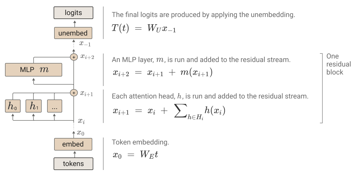
Figure 1. From token embedding through residual blocks to the unembedding. Attention heads and MLPs each add their results into the residual stream.
The residual stream: a conduit that does nothing
At the center of the redrawn picture is the residual stream. Each layer reads its input from the stream and adds its result back. The stream itself has no nonlinearity. It is shared memory with only reads and adds, a communication channel used by all layers together.
The power of this view comes from linearity. A layer’s output stays added into the input of every later layer. So the interaction between two distant components can be summarized by a single product of weight matrices, skipping the layers in between. The paper calls these virtual weights. For example, the direct path from embedding straight to unembedding is one matrix: $W_U W_E$.
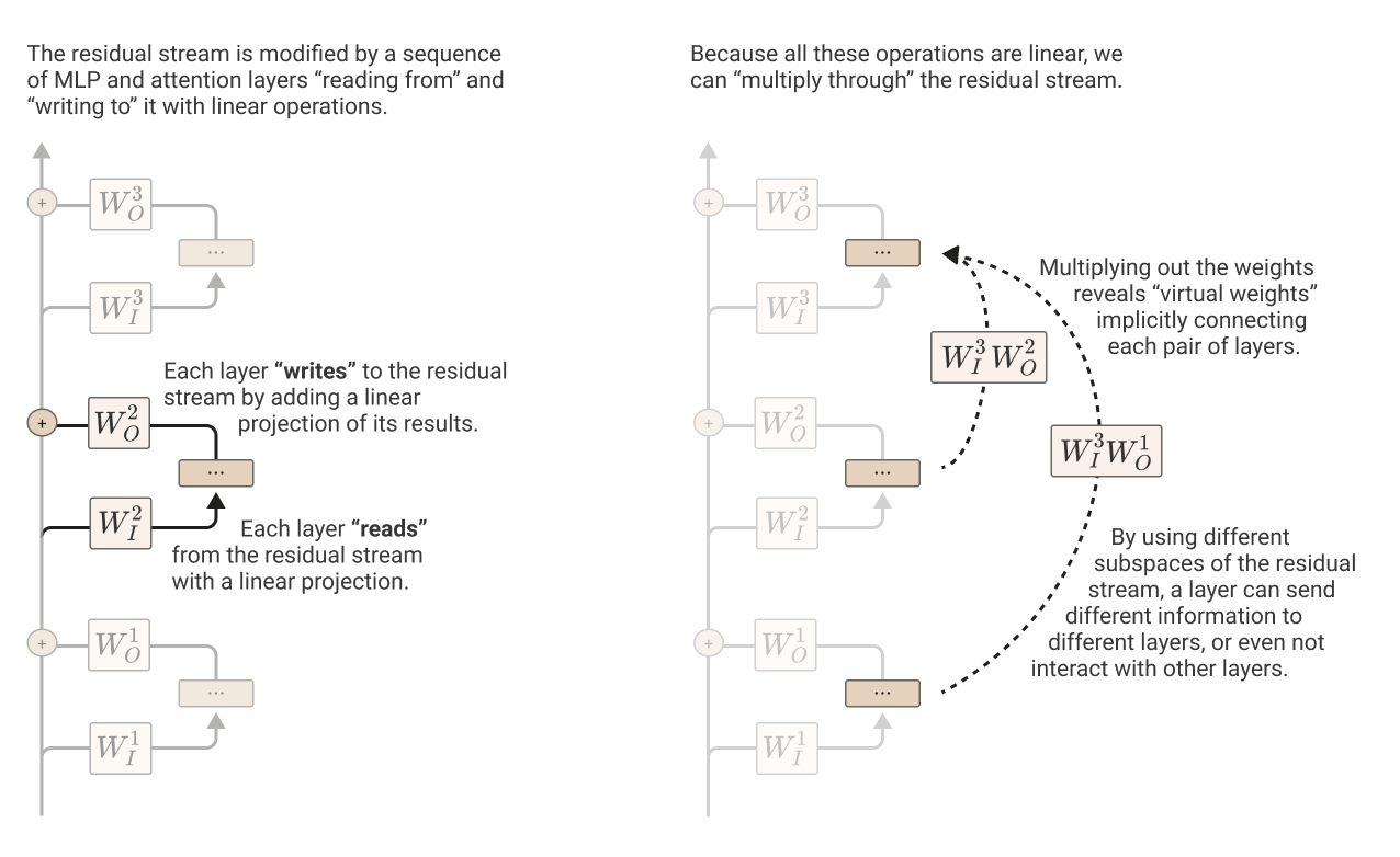
Figure 2. Left: each layer reads from the residual stream and writes back by adding, both with linear maps. Right: because everything is linear, multiplying the weights through reveals virtual weights implicitly connecting each pair of layers. By using different subspaces, a layer can send information to specific layers only.
Another consequence of linearity: the residual stream has no privileged basis. Rotate every matrix that interacts with the stream together, and model behavior is unchanged. It is a space where no individual coordinate axis should be expected to mean anything.
Note: what is a privileged basis? Coordinate axes acquire meaning when some operation applies per axis, the way an activation function does. MLP activations, for example, get a nonlinearity per neuron, so the axis “neuron 3” is a real unit of computation: such a space has a privileged basis. The residual stream, by contrast, is only ever read and written linearly, so rotating the whole space changes nothing about the computation. No axis is special, and the question “what does dimension 137 mean?” is not even well posed. To find meaning, look at directions, linear combinations of dimensions, rather than axes.
The cramped channel: bottleneck, and a preview of superposition
A transformer has exactly one shared, fixed-size memory that every layer uses: the residual stream. What has to fit in it is far larger than it is. So multiple pieces of information end up stored on top of each other in the same space, and this becomes one of the biggest reasons transformers are hard to interpret. That one paragraph is this whole section. Now let’s unpack it, one step at a time.
The residual stream has a finite dimension. In a model with hidden dimension 4096, the stream is a single vector of length 4096. One whiteboard with room for 4,096 numbers is the only channel information travels through. Layers share it by splitting it into subspaces, bundles of slots, rather than using the whole board.
Now count who wants to write. Thousands of attention heads; hundreds of thousands of MLP neurons. The neurons of a single MLP layer alone are typically four times the stream’s dimension. Everyone lines up saying “my result needs to go on the board too,” and the board has 4,096 slots.
Hence the bottleneck. Look at the residual stream around layer 25 of a 50-layer model. Everything the previous 25 layers computed passes through this one vector. Add up the neurons before it: around 400,000, a hundred times the stream’s dimension. In road terms, a hundred lanes merging into four and fanning back out to a hundred. The paper calls such tensors bottleneck activations and expects them to be unusually hard to interpret.
How do 400,000 results fit into 4,096 numbers? The concept previewed here is superposition. One dimension of the stream need not carry only “dog”: it can carry dog plus grammar plus sentiment plus context all at once, the way a single audio signal carries many frequencies mixed together. Even a lone number like 2.31 in the vector can have several meanings folded into it. The follow-up paper Toy Models of Superposition takes this on directly.
And a crowded space needs cleaning. The paper also suggests some heads may play a memory management role: judging “this information is no longer needed” and clearing it from the stream. Not just heads that write and heads that read, but perhaps heads that erase.
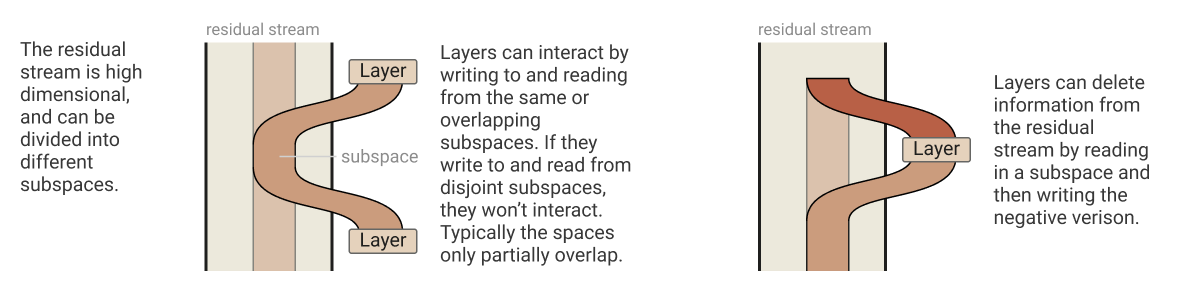
Figure 3. The high-dimensional residual stream divides into subspaces. Layers interact through overlapping subspaces and stay independent in disjoint ones. As on the right, a layer can also delete information by reading a subspace and writing back its negative.
Heads are independent and additive
An attention layer has several heads. In implementations, head outputs are concatenated and multiplied by one big matrix, but mathematically this is equivalent to each head computing independently and adding into the residual stream.
$$\text{AttnLayer}(x) = x + \sum_{h} h(x)$$The layer is a unit of implementation convenience. The natural unit of analysis is the head.
The QK circuit and the OV circuit
A single attention head is really a device answering two independent questions. Where to look. What to take from there. Because attention is usually taught as the computational procedure of queries, keys, and values, the two look like one lump; the paper’s reinterpretation is that two mutually independent functions are merely bundled together. This decomposition becomes the lever for everything that follows.
A concrete example. The model has read “Tom likes apples. He …” and is about to predict the next token. An attention head moves in two steps.
Step one: where to look. The current token “He” issues a search query, and the earlier tokens each carry an index (key). Matching the query against the indexes gives scores, and the softmax turns them into the attention pattern.
Tom     0.93
likes   0.02
apples  0.05
All this step decides is “look at Tom.” Whether Tom is a person, male, or the subject appears nowhere here. Only where to look.
Step two: what to take. Tom it is. But the residual stream at Tom’s position carries layers of information: person, male, subject, a name, singular. The head does not move all of it; it picks out its own share. It might extract just “third person singular,” transform it, and write it into the residual stream at “He.” Exactly the information that makes the next prediction eats rather than eat.
By analogy, step one is the navigation system and step two is the delivery driver. Choosing which house to drive to and choosing which box to load are different jobs.
Now the two steps as matrices. Four matrices $W_Q, W_K, W_V, W_O$ do the computation, and none of them means anything alone. $W_Q$ and $W_K$ always travel together in step one; $W_V$ and $W_O$ always travel together in step two. So the real objects are two products.
The QK circuit $W_{QK} = W_Q^\top W_K$: a table giving, for every token pair, one score for how much this query is drawn to this key. All of step one collapses into this single table.
The OV circuit $W_{OV} = W_O W_V$: a table of how the output is affected if this token gets attended to. All of step two collapses into this single table.
Keep a sense of scale too. With a 4096-dimensional stream and a 128-dimensional head, $W_{QK}$ acts like a 4096 x 4096 table but has only rank 128 of real freedom. However large it looks, the substance is two small low-rank matrices. When part 4 actually reads these tables, this fact is what makes the computation feasible.
From this viewpoint, the key, query, and value vectors are by-products. Factor the two matrices differently and you get entirely different intermediate vectors, yet the model behaves identically. That is why the paper says it is often useful to describe transformers without referring to these vectors at all.
The payoff of the decomposition shows in combinations. Two heads with the identical QK circuit, “always look at the previous token,” are entirely different heads if one’s OV moves part-of-speech information and the other’s moves sentiment. Conversely, with the same OV, changing the QK among previous-token, subject, same-word, and start-of-sentence again gives completely different heads. A head’s function is the combination of its two circuits, which is why describing a head takes two sentences: “this head looks at the previous token” describes its QK, and “this head passes along grammatical information” describes its OV.
The separation is also the analytical lever. Once it is settled where to attend, the delivered effect is a function of the source token alone, so the two tables can be read independently. Reading skip-trigrams off tables in part 4, and predicting their bugs, runs entirely on this. And once this decomposition feels natural, part 5’s induction head becomes easy too: it reads as a combination where the QK walks to the spot of “my previous occurrence” and the OV copies the token next to it.
Hence the paper’s slogan: attention is information movement. A head is a device that reads information from the residual stream at one position and moves it into the residual stream at another.
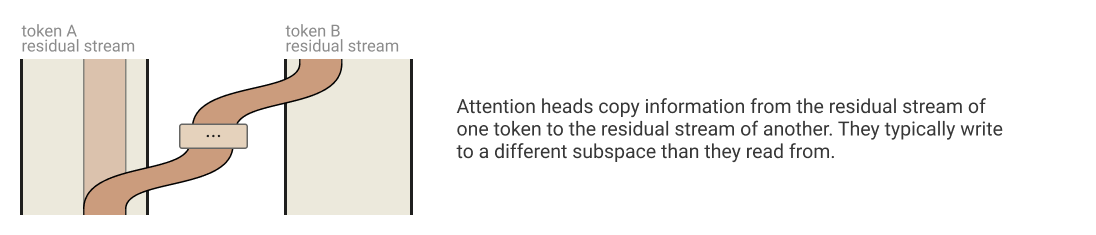
Figure 4. An attention head copies information from one token’s residual stream into another’s, typically writing to a different subspace than it read from.
One more important fact to add. In an attention-only model, the only nonlinearity is the softmax that produces the attention pattern. So the moment the pattern $A$ is treated as fixed, everything else in the model is linear. The path expansion used from the next post on stands exactly on this fact.
Takeaways
- The residual stream is a linear, non-computing communication channel, and its linearity is what makes virtual-weight analysis possible.
- The unit of analysis is the head, not the layer. Heads are independent and additive.
- A head decomposes into where to look (QK) and what to move (OV).
- The only nonlinearity is the softmax. With patterns fixed, the model is linear, and that is what licenses path expansion.
- The stream is one cramped memory shared by everyone; overlapped storage, superposition, is previewed here.
Next up: the smallest model of all, the zero-layer transformer.
Source: the Transformer Overview section of A Mathematical Framework for Transformer Circuits. All figures in this post are from the original paper.