This is the first lecture in a series following David Silver’s UCL reinforcement learning course. Keeping to the order of the slides, we start by defining the problem of reinforcement learning itself.
Lecture slides: PDF
The many faces of reinforcement learning
It is easy to treat reinforcement learning as one technique among many in machine learning, but Silver opens the lecture from the opposite side. Reinforcement learning is just the name computer science gave to a far older and broader question: how do we make good decisions over time?
The same question recurs across many disciplines, each under its own name.
- In computer science, machine learning.
- In engineering, optimal control.
- In neuroscience, the brain’s reward system, that is, dopamine signals.
- In psychology, classical and operant conditioning.
- In mathematics, operations research.
- In economics, bounded rationality and game theory.
Silver’s slide draws these fields as spokes around reinforcement learning at the hub. It is a picture of people who set out from different neighborhoods and arrive, in the end, at the same problem: the science of decision making. This is why reinforcement learning feels so fundamental. It is not a newly invented trick but an old question, one that several disciplines had circled separately, brought together in one place.
What makes reinforcement learning different
Compared with supervised learning, reinforcement learning is missing a great deal.
- There is no supervisor to give the right answer. There is only a reward signal.
- Feedback is not instantaneous but delayed. Today’s choice returns as a consequence only much later.
- The data is not independent. It is sequential data with a temporal order.
- The agent’s actions change the data it will later receive.
In other words, reinforcement learning is not a problem of getting the answer right, but of finding good behavior through trial and error.
Reward, and the reward hypothesis
The reward $R_t$ is a scalar signal that tells the agent, at each time step, how well it is doing. The goal of reinforcement learning is simple: to maximize cumulative reward.
The reward hypothesis nails this down in a single sentence: “All goals can be described as the maximization of expected cumulative reward.” Whether winning a game or making a robot walk, the claim is that goals which look nothing alike all translate into a single reward signal.
That reward is delayed is also central. Often the agent must give up an immediate reward to take a larger one in the distant future.
Example: turning goals into rewards
Since the reward hypothesis can sound empty, let us look at Silver’s examples one by one, through the lens of reward design. What matters is how goals that look utterly different get carried over into a single reward.
- Helicopter aerobatics: + for following the desired trajectory, a large − for crashing. Dense reward can be given at every instant from the trajectory error, which makes learning comparatively smooth.
- Beating the world champion at backgammon: +1 for a win, −1 for a loss, 0 otherwise. Because the reward comes only at the end of the game, delayed and sparse, credit assignment, tracing which move contributed to the win, is hard.
- Managing an investment portfolio: + at each time step by the amount the balance grew. An immediate and natural reward, but without carrying risk the agent drifts toward strategies close to gambling. This is where what has been left out of the reward becomes the problem.
- Controlling a power plant: + for producing power, − for exceeding safety limits. The goal is not a single one; performance and safety must be weighed within one reward. Dissolving a constraint into a negative reward is a common design.
- Making a humanoid robot walk: + for moving forward, − for falling. It looks simple, but rewarding only “forward” makes it easy to exploit the reward by, say, toppling forward. It is a good example of the pitfall of reward shaping.
- Playing Atari games better than a human: + when the score rises, − when it falls. There is the convenience of reusing a game’s existing score, but when the score diverges from the true goal, behavior that only feeds on the score can appear.
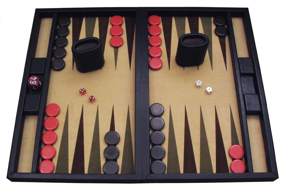
Backgammon. A two-player board game in which the two players roll dice and move their fifteen pieces each in opposite directions, the first to bear them all off winning. Since the outcome is decided only at the end, the reward is delayed. (Photo: Ptkfgs, public domain)
The lesson running through all six is this. In reinforcement learning, the most creative and most dangerous work is not the learning algorithm but setting the reward. Translate the goal wrongly, and the agent achieves to perfection not what we wanted but what we wrote down.
As an aside, the Atari case at the end of the list was no distant matter for Silver. That result, “seeing only pixels and score, playing several games better than a human,” is precisely the DQN (Deep Q-Network) work from DeepMind, where Silver was. It was published as a 2013 workshop paper and a 2015 Nature paper, and a single neural network learned dozens of Atari games from raw screen and score alone, without relearning each game’s rules. This demo is often cited as the scene that led Google to acquire DeepMind in 2014. So when Silver raises this example in lecture 1, he is quietly pointing at his own team’s result, the one that announced deep reinforcement learning to the world. This DQN is the value function approximation of lecture 6, and its line runs on to AlphaGo in lecture 10.
Agent and environment, and state
At each time step $t$ the agent takes an action $A_t$, and the environment returns an observation $O_t$ and a reward $R_t$. The record of this exchange strung together from the beginning is the history.
$$H_t = O_1, R_1, A_1, \dots, A_{t-1}, O_t, R_t$$Not only the observations and rewards but the agent’s own past actions (the $A$’s) are all held within it, the whole sensorimotor stream of the robot, so to speak. What happens next depends on this history.
But we cannot carry the entire history around every time. The summary that keeps only the information needed for the next decision is the state, defined as a function of the history: $S_t = f(H_t)$. What matters here is that how to choose $f$ is the designer’s choice.
Here it is worth distinguishing observation from state. The observation $O_t$ is a single raw scene the agent received at that instant. The state $S_t$ is not that one scene but the information distilled from the history so far and used for the next decision. It is rare for a single observation to become the state as it is. Just as one frame of a game screen cannot even tell where the ball is moving, it usually takes several observations woven together to make a state. The observation being the state itself holds only in the special case of full observability, seen later.
Three kinds of state
The same situation is viewed from three perspectives.
- Environment state $S^e_t$: the representation the environment holds internally. It is the data the environment actually uses to determine the next observation and reward. It is usually not visible to the agent, and even when visible it may be laced with a great deal of information irrelevant to the decision.
- Agent state $S^a_t$: the internal representation the agent uses to choose its next action. This is what the reinforcement learning algorithm actually grasps. It can be anything that is a function of the history: $S^a_t = f(H_t)$.
- Information state (Markov state): a state that holds, without remainder, the useful information from the history.
The difference between environment state and agent state is sharpest if you picture a classic game emulator. Inside the emulator is the memory (RAM) that fully determines the game at that instant: enemy coordinates, remaining lives, and even internal variables that never show on screen. This is the environment state, and what the game does next depends entirely on it. What a person or an agent actually sees, on the other hand, is only the screen pixels. The pixels are a shadow cast by that memory, so the screen alone cannot fully recover the hidden variables. What the agent distills for itself from that screen is the agent state. So if it sees only the screen it is partial observability, and if it can read the emulator’s memory whole it is full observability. The Atari DQN from earlier stands precisely on the partial-observability side, seeing only pixels and stacking several frames to make its own state.
The Markov state satisfies this condition.
$$\mathbb{P}[S_{t+1} \mid S_t] = \mathbb{P}[S_{t+1} \mid S_1, \dots, S_t]$$It means that knowing the present state alone makes the prediction of the future the same as knowing the entire past. The state is a sufficient statistic of the future, so once the state is known the history may be discarded. The environment state and the history itself are always Markov.
Go is a good example. Given only the arrangement of stones on the board now, that is enough to decide the next move, and it does not matter in what order that arrangement was reached. So the current state of the board is a Markov state. (Strictly, a little history is needed because of repetition-forbidding rules like ko, but in the big picture the board now is the state.)
Extracting state from history: the rat experiment
Silver’s rat example shows well why how you define the state matters. In front of a rat, a light and a bell turn on and the rat presses a lever, following in some order, and at the end comes cheese (good) or an electric shock (bad). Even for the very same history, the prediction diverges depending on how the state is taken.
- What if state = the last three items?
- What if state = the counts of how many times light, bell, and lever each appeared?
- What if state = the whole sequence as it is?
The three yield different futures. Under one representation cheese may be predicted, under another the shock. In reinforcement learning, “how you define the state” determines “what you can predict.” Finding a good state representation is itself half the problem.
One more thing is tangled in here. The history holds not only what the rat saw (light, bell) but also what the rat did (pressing the lever). Whether to include or discard these past actions when extracting the state is also part of the design. If lever presses go into “the last three items,” the state carries a memory of its own actions; if only counts are kept, order information is discarded. Usually past actions help in gauging the future, so they are included in the state.
Full and partial observability
How much of the environment can be seen divides two worlds.
Full observability is the case where the agent sees the environment state directly. Observation = agent state = environment state = Markov state, and this is the Markov decision process (MDP), the protagonist of the next lecture. Go is like this. The whole board is visible to both players.
Partial observability is the case where the agent sees the environment only indirectly. In poker the opponent’s cards are hidden, so what I see (my cards, the board cards, the betting record) is only part of the actual game. A robot seeing the world through a single camera, or a trading agent seeing only the current price, is the same. Now the agent state and the environment state split apart, and this is called a partially observable Markov decision process (POMDP). The agent must fill in what is hidden and build a state for itself. There are several methods: using the history whole, maintaining a belief (a probability distribution) about the environment state, or summarizing the past with a recurrent neural network.
The three pieces that make up an agent
A reinforcement learning agent consists of some or all of the following three.
- Policy $\pi$: the rule from state to action. Deterministic, $a = \pi(s)$; stochastic, $\pi(a \mid s) = \mathbb{P}[A_t = a \mid S_t = s]$.
- Value function: a function that rates how good a given state is going forward. It is the expected sum of future rewards.
Here $\gamma \in [0,1]$ is the discount factor, which sets how much the distant future is discounted.
- Model: the agent’s prediction of how the environment will behave. It consists of the transition $\mathcal{P}$, which foresees the next state, and $\mathcal{R}$, which foresees the next reward.
Which of these three an agent is equipped with is how we categorize it. Using only the value function is value-based, only the policy is policy-based, both is actor-critic. Using no model of the environment is model-free; building a model and planning is model-based.
Silver draws these three onto a single maze. On the same maze, the policy shows up as arrows for where to go from each cell, the value function as a number for how close each cell is to the goal, and the model as how the cells connect and what reward each cell carries. One problem drawn three ways.
The three fundamental questions of reinforcement learning
The lecture closes with three pairs of distinctions that run through reinforcement learning.
- Learning vs. planning: does the agent learn by interaction without knowing the environment (learning), or does it know a model of the environment and turn it over in its head to find the answer (planning)?
- Exploration vs. exploitation: does the agent try something new to gain information (exploration), or take the best it knows so far (exploitation)? This balance is the core of what makes reinforcement learning hard.
- Prediction vs. control: the problem of evaluating how good a given policy is (prediction), and the problem of finding the best policy (control).
Silver contrasts learning and planning with Atari. The learning side plays directly without even knowing the rules of the game, revising its policy on the reward of the score alone. The planning side assumes it holds a perfect model, the emulator, and, without actually operating anything, turns over “what happens if I press this button” inside that model in advance to find the best move. The earlier story of the emulator returns here.
From the next lecture on, we enter the framework for treating this problem mathematically: the Markov decision process (MDP).