Trajectory ML 02: PCA as the First Latent Space

PCA chooses a flat coordinate system that preserves as much variation as possible. It is a useful first representation because its objective is explicit, its solution is inspectable, and its failures are easy to demonstrate.

Imagine two measured features rising together. Points form a long diagonal cloud. Reporting both coordinates repeats much of the same information; reporting position along the long axis retains most of the variation. The perpendicular distance records what that one-coordinate description loses. PCA makes this tradeoff precise.

Preparation and class plan

You need matrix multiplication, dot products, and the idea of a derivative. We introduce eigenvectors rather than assuming mastery. Allocate 15 minutes to a two-dimensional cloud, 30 to the derivation, 15 to SVD, 20 to the lab, and 10 to interpretation. The deliverable is a reconstruction curve plus a justified choice of dimension.

Use the environment instructions, complete lab bundle, and lesson02.py. The same synthetic sessions continue from lecture 1.

Center before choosing a direction

Let $X\in\mathbb R^{n\times D}$ contain training observations as rows. Define the training mean $\mu$ and centered matrix

The diagonal entry $S_{jj}$ is feature $j$’s sample variance. The off-diagonal entry $S_{jk}$ is sample covariance: positive values indicate that two centered features often have the same sign. Covariance has units, so a feature measured in large numerical units can dominate.

For a concrete toy, let

Along $(1,1)/\sqrt2$, the variance is 7; along $(1,-1)/\sqrt2$, it is 1. The first direction captures $7/8$ of total variance. A student should be able to verify both statements with two matrix-vector products. An eigenvector is exactly a direction that the covariance matrix scales without rotating: $Sw=\lambda w$.

Centering matters because PCA describes variation around the mean. Without it, the direction from the origin to the cloud can dominate. Scaling is a separate choice. In the lab we standardize each feature with training statistics so no unit wins by default. This means we optimize reconstruction in standardized units, not raw feature units. The scikit-learn PCA guide confirms that PCA centers inputs but does not itself scale them.

Derive reconstruction PCA

Choose $d$ orthonormal directions as columns of $W\in\mathbb R^{D\times d}$, so $W^\top W=I_d$. Encode observations in $Z\in\mathbb R^{n\times d}$ and reconstruct them as $ZW^\top$:

For fixed $W$, differentiating with respect to $Z$ gives $Z=X_cW$. The reconstruction is the orthogonal projection $X_cWW^\top$. Substituting it back gives

The first term is fixed. Minimizing lost energy therefore maximizes retained variance. For one component, maximize $w^\top Sw$ subject to $w^\top w=1$. A Lagrange multiplier yields $Sw=\lambda w$; the largest eigenvalue gives the maximum. Subsequent orthogonal directions take subsequent eigenvectors.

For our toy, retaining one axis loses variance 1. Retaining both loses zero. Zero training reconstruction error at full dimension does not mean a model discovered useful structure: it merely means it preserved everything, including noise.

Why the implementation uses SVD

Factor the centered matrix directly:

Then $X_c^\top X_c=V\Sigma^2V^\top$. Thus the top right singular vectors are PCA directions, the scores are $Z=U_d\Sigma_d$, and the explained variances are $\lambda_j=\sigma_j^2/(n-1)$. This is a relationship between two decompositions of the same centered data, not a second unrelated algorithm.

The best rank-$d$ reconstruction has squared error

This identity is useful for debugging. The lab compares reconstruction error with discarded singular-value energy and compares the SVD projection with scikit-learn’s projection. Compare projections rather than raw eigenvectors: changing the sign of an eigenvector gives the same subspace, and repeated eigenvalues allow rotations within a tied eigenspace.

Python implementation and honest evaluation

This is the central implementation in the downloadable lab:

from common import make_dataset
from sklearn.preprocessing import StandardScaler
from sklearn.decomposition import PCA

data = make_dataset()
train = data["train"]
scaler = StandardScaler().fit(data["X"][train])
X = scaler.transform(data["X"])
pca = PCA(n_components=2, svd_solver="full").fit(X[train])
Z = pca.transform(X)
reconstruction = pca.inverse_transform(Z)
print(((X[~train] - reconstruction[~train]) ** 2).mean())

The script also sweeps dimensions 1 through 24 and saves the following diagnostic. Run python lesson02.py --output outputs from the bundle directory.

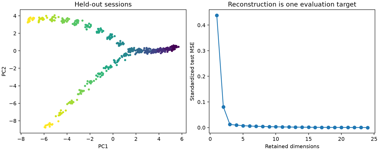
Fitting the scaler before splitting would leak held-out distribution information. Fitting PCA on every row would do the same, even without labels. This course uses an inductive protocol: learn a representation on training sessions and transform new sessions with fixed parameters.

The curve is for understanding compression, not repeatedly selecting a model on a supposedly untouched test set. In a real study, select dimension using training cross-validation or a separate validation group, then evaluate the chosen procedure once on test groups. Report error in the units you actually optimized. inverse_transform here returns standardized observations; apply the scaler’s inverse transform to recover original units.

From measurements to interpretation

In gene-expression analysis, a large-variance axis might reflect differentiation, library size, cell cycle, or technical batch. PCA does not know which is scientifically relevant. Appropriate count preprocessing and experimental metadata are necessary before naming an axis. Inspect loadings and independent markers; do not call PC1 “developmental time” merely because it looks smooth.

For character conversations, an axis might separate confrontation from cooperation, or merely long messages from short ones. A feature’s large loading tells us how it contributes to this linear axis, not that the feature causes the narrative outcome. Context construction and feature scaling shape the answer before PCA begins.

A two-dimensional picture can hide a branch separated mainly on PC3. Choose visualization dimension and modeling dimension separately. High explained variance is evidence of compression under this objective; it is not evidence that the endpoint-relevant signal survived.

Exercises with checks

1. Verify the toy. Multiply the covariance matrix by both unit directions. Answer: eigenvalues 7 and 1, retained fraction $0.875$, discarded variance 1.
2. Change measurement units. Multiply one raw feature by 100 and run PCA with and without standardization. Hint: raw covariance gives that feature much more influence; standardized PCA should be unchanged up to numerical and sign differences.
3. A tiny but decisive feature. Imagine an outcome depends only on a low-variance axis. Is keeping 95% of variance sufficient? Answer: no. A representation objective and a prediction objective can disagree. Evaluate the downstream task using valid splits instead of treating 95% as a universal rule.

PCA gives a strong baseline precisely because we can state what it preserves. The next lecture changes the map from linear to nonlinear while keeping reconstruction as a starting objective.