Trajectory ML 03: Autoencoders, VAEs, and Useful State

A nonlinear encoder can compress a curved dataset that a straight PCA subspace describes poorly. It does not automatically discover the concepts we care about. This lecture makes both points visible by training a PCA baseline, an autoencoder, and a variational autoencoder on the same observations.

Imagine points on a bent strip in two dimensions. A single straight projection may place distant sections of the strip on top of each other. A nonlinear encoder can assign a coordinate that follows the bend, while a decoder maps that coordinate back to the strip. The gain comes from changing the shape of the map, not from adding biological or narrative understanding.

Preparation and 90-minute plan

Review PCA reconstruction and the chain rule. You should know what a neural-network layer and gradient descent do. Spend 15 minutes on the curved toy, 20 on autoencoders, 25 on VAE probability, 20 running the lab, and 10 diagnosing representations. The required outcome is a comparison table with separate reconstruction and interpretation claims.

Use the course setup and lab bundle. lesson03.py contains runnable CPU PyTorch implementations. It downloads neither model weights nor data.

An autoencoder learns both maps

An encoder produces $z=f_\phi(x)$ and a decoder reconstructs $\hat x=g_\theta(z)$. With a two-dimensional bottleneck, our model maps 24 input coordinates to two numbers and then back to 24:

In the lab each map contains one hidden layer of 32 units with Tanh. The output decoder is linear because standardized continuous features can be negative. A sigmoid output would impose an inappropriate $[0,1]$ range. The feature likelihood and output activation must match the data, not a copied image tutorial.

A linear autoencoder with appropriate capacity and a squared-error optimum can span the PCA subspace, but its latent axes need not equal PCA axes. Nonlinearity expands the possible reconstructions. It also introduces optimization choices, overfitting, and dependence on initialization. Hinton and Salakhutdinov’s original autoencoder study is useful historical context; the small network here is a teaching implementation, not a reproduction of that training procedure.

An encoder can faithfully retain nuisance variation. If speaker identity makes reconstruction easy, the model may prioritize identity over story progress. A reconstruction objective alone cannot know that you wanted a causal or interpretable state.

A VAE represents uncertainty with a distribution

Suppose several latent states could plausibly explain one noisy observation. Instead of emitting one code, the encoder emits a distribution

We choose a prior $p(z)=\mathcal N(0,I)$ and an observation model $p_\theta(x\mid z)$. In this lab the observation model is Gaussian with decoder mean and fixed standard deviation $s=0.3$ in standardized feature units. The network outputs logvar, the logarithm of latent variance, which is distinct from that observation noise.

A VAE maximizes the evidence lower bound:

$$ \mathcal L(x)=\mathbb E_{q_\phi(z\mid x)}[\log p_\theta(x\mid z)]

• D_{\mathrm{KL}}!\left(q_\phi(z\mid x)|p(z)\right) \leq\log p_\theta(x). $$

The first term rewards explaining the observation. The second charges for departing from the prior. KL is not an arbitrary punishment for “complicated” pictures: it compares two distributions. The identity

explains why this is a lower bound. The nonnegative gap is the mismatch between the approximate and model posterior. Kingma and Welling’s original paper develops this variational objective and its gradient estimator.

For a diagonal Gaussian, the prior KL has a closed form:

Set $\mu=0$ and $\ell=0$: the distributions match and KL is zero. This is an easy unit-level mathematical check, even before training.

Sampling that still permits gradients

We sample $\epsilon\sim\mathcal N(0,I)$ and write

Randomness now sits in $\epsilon$; differentiable operations connect the sampled code to network outputs. This is the reparameterization trick. In the full code, reconstruction uses this sampled code during training. The per-observation negative objective, omitting a parameter-independent constant, is

Notice the sum over features before averaging across observations. Accidentally averaging one term over features but summing the other changes their relative weight. Our code uses an ordinary ELBO with fixed observation noise, not an unlabeled beta-VAE objective. Choosing $s$ still changes the reconstruction-versus-prior tradeoff.

Run and read the comparison

From the extracted directory, run this executable excerpt:

from common import make_dataset
from lesson03 import train_models

data = make_dataset()
embeddings, metrics = train_models(data, epochs=300)
for name, value in metrics.items():
    print(name, value)

For the figure, run python lesson03.py --output outputs. The file includes both model classes, the exact loss, fixed seeds, and training-session-only standardization. Test sessions influence neither weights nor preprocessing. The small full-batch training loop makes every operation inspectable; production training would usually use minibatches and validation-based stopping.

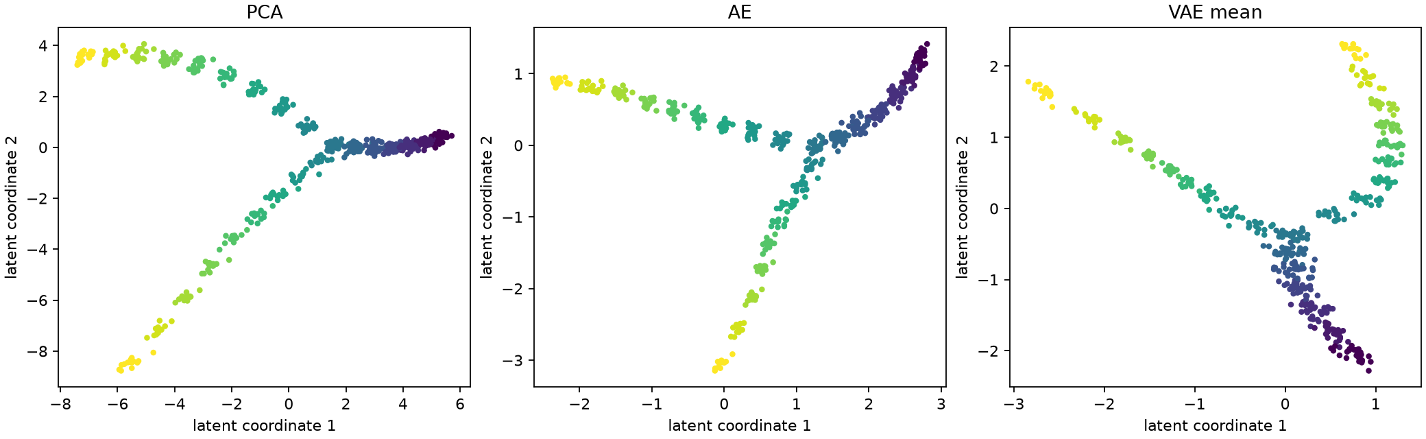
All three plots color held-out observations by recorded time for inspection. They do not train on time or z_true. The VAE plot shows posterior means. Its reported mean-decoder MSE measures reconstruction at $\mu(x)$; it is not the stochastic expected reconstruction term in the ELBO. Reporting those as the same quantity would obscure uncertainty.

A smaller MSE is one result, not an automatic ranking of state quality. Inspect whether nearby sequence steps remain nearby, whether held-out branch information remains recoverable, and whether nuisance labels dominate. If you tune architectures after inspecting test results, create a fresh untouched test set for final reporting.

Biology and character dialogue

For gene counts, a Gaussian squared-error model may be a poor measurement model; count-aware likelihoods and library-size handling can matter. The synthetic features here are continuous on purpose. A visually neat latent map alone does not validate cell identities or developmental ordering.

For dialogue, reconstructing a pretrained embedding preserves what that embedding encodes. It cannot recover a forgotten fact that the context window never contained. Evaluate a state representation with future-turn or outcome tasks using only information available at prediction time, and inspect behavior across users and characters.

Latent sampling is also not narrative uncertainty calibration. A VAE may be confidently wrong under domain shift; a smooth prior is not evidence that all intermediate decoded states are meaningful. Unsupervised axes are generally not uniquely identified as semantic factors without additional assumptions, as discussed by Locatello et al..

Exercises and answer hints

1. Remove the bottleneck. Increase latent dimension to 24. Why might training MSE improve without better state discovery? Answer: the model has more room to copy observations and noise. Check held-out tasks, not just reconstruction.
2. Compute a KL term. For one latent coordinate with $\mu=1$ and $\sigma^2=1$, what is KL to $\mathcal N(0,1)$? Answer: $1/2$. With $\mu=0,\sigma^2=1$, it is zero.
3. Change observation noise. Compare $s=0.15$ and $s=0.6$ with a validation split. Hint: the smaller $s$ assigns more weight to reconstruction. Record both MSE and KL; neither alone measures semantic usefulness.

Next we change the question from reconstructing each observation to preserving neighborhoods on a curved space.