Two observations can be close in the surrounding space yet far apart along the surface on which data actually vary. Manifold learning starts by deciding which local connections are trustworthy, then uses those connections to construct a larger picture.
Think of a sheet of paper rolled into a Swiss roll. Points on neighboring layers can nearly touch through the air. To walk between them while staying on the paper, however, you may need a long trip around the roll. A straight-line distance and a surface distance answer different questions.
Preparation and lesson plan
Review PCA, pairwise distance, and a graph’s nodes and edges. Spend 15 minutes on the rolled-paper example, 20 building nearest-neighbor graphs, 20 on Isomap, 15 on UMAP, and 20 running and diagnosing the lab. Your final explanation should distinguish ambient dimension, intrinsic dimension, and visualization dimension.
Use the course setup, complete bundle, and lesson04.py. The script needs umap-learn as well as scikit-learn. The first UMAP execution may take longer because its numerical routines compile locally.
A surface is not a curve
A standard Swiss roll can be parameterized by
$$ x(u,v)=(u\cos u,\ v,\ u\sin u). $$It has three observed coordinates but two free parameters, $u$ and $v$. Its intrinsic dimension is two. Unrolling it should produce a two-dimensional sheet, not a one-dimensional time line. A single spiral curve drawn on that sheet would be a different, one-dimensional dataset.
Even $(u,v)$ is not automatically an isometric coordinate system: moving along $u$ has speed $\sqrt{1+u^2}$. Surface arc length requires integrating that speed. This detail helps explain why recovering an unrolled sheet does not require an algorithm’s horizontal axis to equal the generator’s $u$ values.
The manifold hypothesis says that high-dimensional observations can concentrate near a lower-dimensional structure. It is a modeling hypothesis, not a guarantee about every dataset. Branch points, disconnected populations, sharp changes, and mixtures can violate a single smooth-manifold description. Our branching trajectory data already remind us that a graph may be more appropriate than one global smooth chart.
Build the local graph first
For each point, find its $k$ nearest neighbors using the chosen feature-space metric. Connect those neighbors and weight an edge with their Euclidean distance. Because “$j$ is among $i$’s neighbors” need not imply the reverse, symmetrize the graph. In this lab an edge exists when either direction chooses it.
$$ d_G(i,j)=\min_{\pi:i\leadsto j}\sum_{(a,b)\in\pi}\|x_a-x_b\|_2. $$This shortest-path distance approximates a surface geodesic when samples are sufficiently dense and local edges remain local. It does not become reliable merely because a shortest-path algorithm returned a number.
The choice of $k$ creates a tradeoff. Too few neighbors can disconnect the graph or fragment a sparse region. Too many can bridge different layers of the Swiss roll or connect biological branches that are separate. Standardization, noise, and sampling density affect the same decision. Inspect connectivity and repeat the analysis over a reasonable neighborhood range.
Isomap: preserve graph distances
Isomap constructs the neighbor graph, computes shortest paths between all training points, and embeds those distances using classical multidimensional scaling. If $D_G$ is the matrix of graph distances and $H=I-\mathbf1\mathbf1^\top/n$, define
$$ B=-\frac12H(D_G\odot D_G)H. $$For an exactly Euclidean distance matrix, $B$ is a centered Gram matrix. Its top positive eigenpairs give coordinates $Y=V_d\Lambda_d^{1/2}$. With estimated geodesics, this becomes an approximation and negative eigenvalues can occur. You have met the eigenvector operation before; what changed from PCA is the matrix being decomposed.
The original Isomap paper by Tenenbaum, de Silva, and Langford formalizes the connection between local neighborhoods and global geometry. For implementation behavior, including transformation of new points, consult the scikit-learn manifold guide.
All-pairs graph distances require substantial memory as the dataset grows. Isomap is attractive for this small diagnostic; an exact all-pairs computation is not a default choice for millions of cells or conversation windows.
UMAP: preserve a weighted neighborhood structure
UMAP also begins with neighborhoods, but it does not aim to reproduce the entire Isomap shortest-path distance matrix. It constructs locally scaled fuzzy neighbor memberships, combines them into a graph, and optimizes a low-dimensional arrangement that reflects those memberships. Attractive and repulsive terms help form that arrangement. The original UMAP paper gives the formal construction.
n_neighbors changes the scale of neighborhood structure considered. min_dist influences how tightly points can pack in the output. Consequently, the width of an island or the white space between two islands can change with display choices. Do not turn a plotting gap into a measured biological barrier or a duration of narrative change.
UMAP can be useful for exploratory visualization while leaving global distances, densities, and axis meanings distorted. It does not supply a time arrow. Coloring by known time is a diagnostic, not a conversion of a UMAP coordinate into a clock. Subsequent trajectory analysis should justify the space and graph it uses instead of blindly connecting dots in a display.
The two-part experiment
Run the core experiment from the extracted lab directory:
from common import make_dataset
from lesson04 import fit_manifolds

data = make_dataset()
embeddings, metrics = fit_manifolds(data)
print(metrics)
The helper standardizes features using training sessions only, checks the training graph’s connectivity, fits Isomap and UMAP on training observations, and transforms held-out sessions. It uses 30 neighbors for the shared data. No generator coordinate or time label enters fitting.
Run python lesson04.py --output outputs to add the separate Swiss-roll diagnostic and save the figure. That diagnostic intentionally fits all 800 roll points: it illustrates geometry and is not a claim about held-out generalization. The script reports its connectivity separately from that of the session experiment.
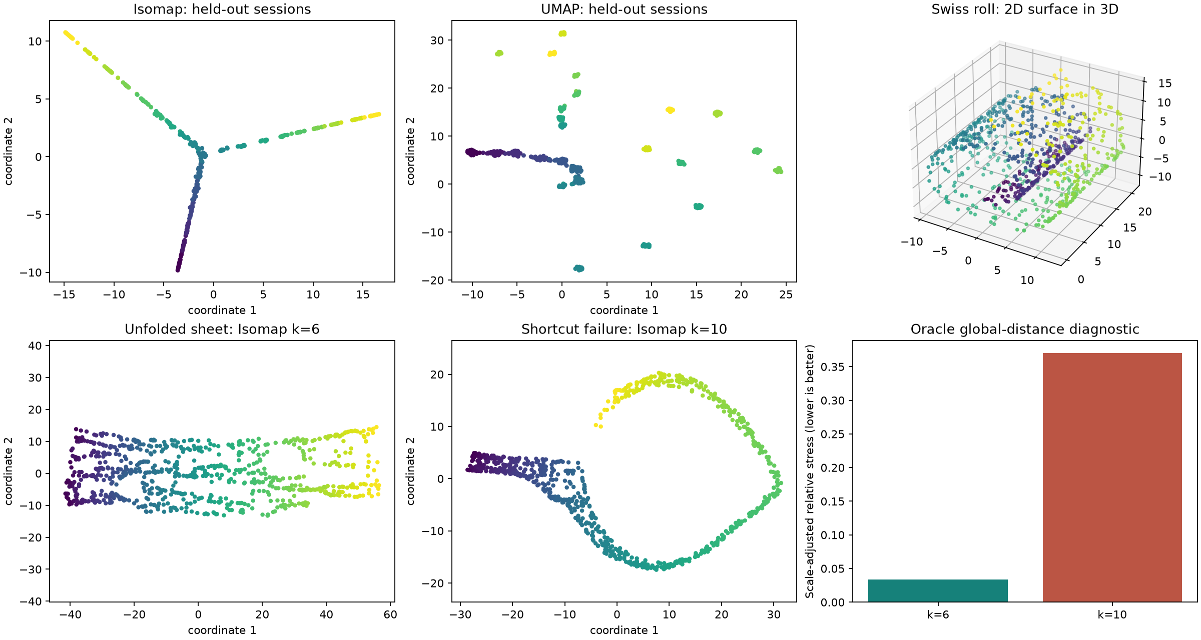
The fixed-seed Swiss-roll experiment compares two connected graphs. With 6 neighbors the sheet unfolds; with 10, five edges cross between distant parts of the sheet and create shortcuts. We flag an edge when its known intrinsic length exceeds twice its observed length. This is a synthetic oracle check, not a rule available for unknown real manifolds.
The last panel reports scale-adjusted distance stress, $\min_{a>0}\sqrt{\sum_{i The shared-data metrics include trustworthiness at 10 neighbors. It penalizes points that become near neighbors in the embedding even though they were distant in the reference feature space. A high score means relatively few such local false neighbors. It does not establish preserved global distances, correct direction, or scientific relevance of the original metric. In this run, UMAP scores about 0.993 while displaying fragmented islands in the shared trajectory. Good local neighborhoods can coexist with a misleading global layout. Complement the score with neighborhood recall, graph connectivity, parameter sensitivity, and independent labels. In cell-state analysis, a smooth curve can reflect differentiation, but it may also reflect a technical gradient. Check donor and batch labels along with independent biological markers. A gap may represent undersampling rather than an impossible transition. Do not infer lineage solely from where UMAP places an island. For character dialogue, semantic similarity can connect different moments: two apologies may occur before and after very different events. A state representation must include enough history for the intended transition question. Inspect consecutive-turn edges separately from similarity edges; temporal adjacency and semantic adjacency need not agree. The reusable lesson is local geometry first, global claims second. Next we will put a random walk on a neighbor graph and ask what repeated local transitions reveal.What each application contributes
Exercises with interpretation checks