A diffusion map places two observations close together when random walks starting from them reach similar neighborhoods. It gives us a global coordinate system built from local connections. This lecture’s transition matrix describes exploration of a dataset, not the actual movement of cells or conversations.
Prerequisites: PCA eigenvectors, distances, conditional probability, and Lecture 4’s kNN graph. 90 minutes: intuition and toy walk 15, matrix construction 20, spectral coordinates 20, Python 25, interpretation 10. By the end, you should be able to construct a valid transition matrix, explain its stationary distribution, and distinguish diffusion time from elapsed time.
Use the shared setup and data contract. Download lesson05.py with the complete lab bundle.
1. A walk along two curved arms
Draw a U in two dimensions. Its tips may be close in Euclidean distance, while traveling through nearby points requires going around the bend. Now place a walker on each tip. After one step, their reachable neighborhoods differ. After many steps, both walkers can explore the whole U.
On the three-node path A–B–C with unit edges, an ordinary walker moves A→B with probability 1, and B→A or B→C with probability 1/2. Its transition matrix is
$$P_0=\begin{pmatrix}0&1&0\\1/2&0&1/2\\0&1&0\end{pmatrix}.$$The middle node receives more visits because it has more incident edges. The stationary probabilities are $(1/4,1/2,1/4)$, not $(1/3,1/3,1/3)$. Also, this graph alternates between two sides. We remove that periodicity with a lazy walk: stay still half the time, otherwise take an ordinary step.
2. Affinity, degree, transition
Let $r_i$ be observation $i$ after scaling and PCA. Connect $i,j$ when either belongs to the other’s $k$ nearest neighbors. On these edges set
$$W_{ij}=\exp(-\|r_i-r_j\|^2/\sigma^2),\quad W_{ii}=0.$$Symmetrize the graph; our implementation takes the maximum of the two directed affinities. Larger $W$ means stronger similarity. Define $d_i=\sum_jW_{ij}$ and $D=\operatorname{diag}(d_i)$. Then
$$P_0=D^{-1}W,\qquad P=\tfrac12(I+P_0),\qquad \pi_i=\frac{d_i}{\sum_jd_j}.$$Each row of $P$ sums to one. For a connected graph, $\pi$ is its unique stationary distribution. Detailed balance, $\pi_iP_{ij}=\pi_jP_{ji}$, means this constructed walk is reversible. It does not mean biological development is reversible.
A graph with disconnected components has no route between them. It has several eigenvectors with eigenvalue one, and the stationary mixture between components is not unique. Inspect connected components before interpreting any map. Isolated nodes require separate handling because division by their degree is undefined.
3. Laplacians and slow coordinates
The combinatorial Laplacian is $L=D-W$. For a scalar value $f_i$ attached to every node,
$$f^TLf=\frac12\sum_{ij}W_{ij}(f_i-f_j)^2.$$A small value says connected nodes have similar values. This explains why low-frequency eigenvectors describe smooth structure. The symmetric normalized Laplacian is
$$L_{\rm sym}=I-D^{-1/2}WD^{-1/2}.$$It is different from $L$; degree normalization changes the problem. For our lazy walk, solve the symmetric matrix $S=I-L_{\rm sym}/2$. If $Su_\ell=\lambda_\ell u_\ell$, its corresponding right eigenvector of $P$ is $\psi_\ell(i)=u_\ell(i)/\sqrt{\pi_i}$. This scaling makes the eigenvectors orthonormal under stationary weights.
Discard the constant eigenvector with $\lambda_0=1$. At diffusion step $t$, coordinates are
$$\Phi_t(i)=\big(\lambda_1^t\psi_1(i),\ldots,\lambda_m^t\psi_m(i)\big).$$Modes with smaller eigenvalues fade faster. Large $t$ emphasizes slow mixing structure but can erase useful detail. The original diffusion-map paper develops this spectral construction and its multiscale interpretation.
The distance being approximated is
$$D_t^2(i,j)=\sum_k\frac{(P^t_{ik}-P^t_{jk})^2}{\pi_k}.$$For a connected reversible walk, retaining all nonconstant eigenvectors makes squared Euclidean distance in diffusion coordinates equal this expression. Keeping two coordinates is a truncation, not an exact preservation of every distance. Ordinary Euclidean distance between rows of $P^t$ omits the stationary weighting.
4. Python: verify the walk before plotting
The script constructs sparse affinities and diagonalizes $S$ with eigsh. The excerpt runs from the extracted lab directory and is also the core computation in the downloadable script:
from common import make_dataset, prepare_embedding
from lesson05 import affinity_graph, diffusion_coordinates
import numpy as np

data = make_dataset()
_, Z, _, _ = prepare_embedding(data, n_components=6)
W = affinity_graph(Z, k=48)
Dmap, values, P, pi, components = diffusion_coordinates(W, time=4)
print(components, values)
print(np.max(np.abs(np.asarray(P.sum(axis=1)).ravel() - 1)))
print(np.max(np.abs(np.asarray(pi @ P).ravel() - pi)))
Run python lesson05.py --output outputs. The JSON reports row-sum and stationarity errors; both should be close to floating-point precision. The PNG compares the first two PCs with diffusion coordinates. Time colors are added after construction and do not enter the graph.
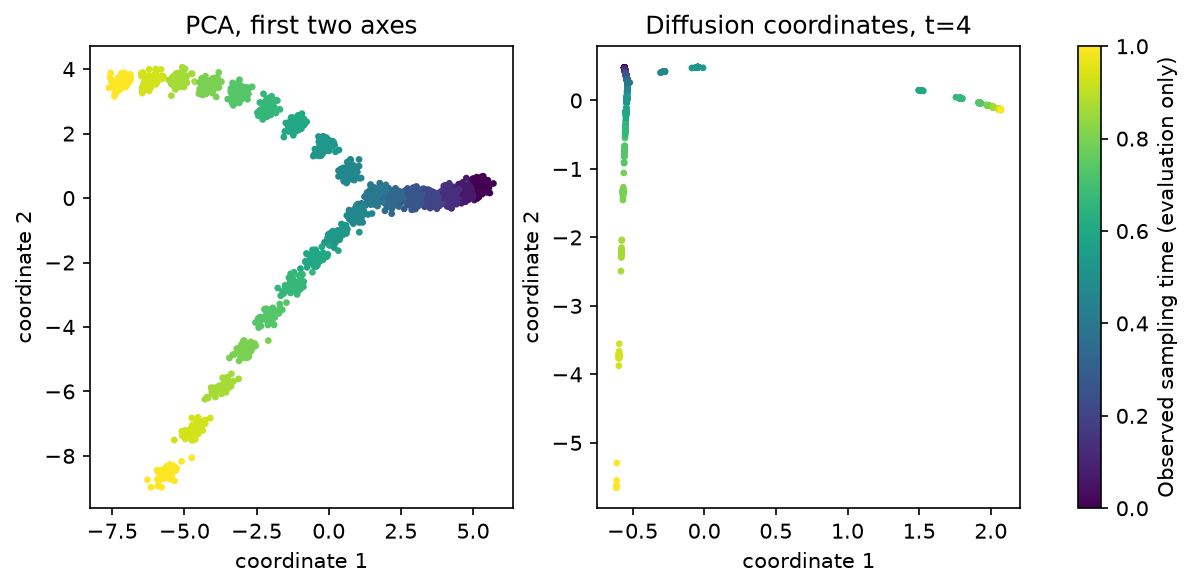
Scaling and PCA are fitted on training sessions. However, this graph contains all observations, including held-out sessions. Its result is a transductive exploratory map. It is not a held-out forecast. An inductive application needs a separately specified extension to new points and an evaluation split appropriate to that task.
5. Cells and conversations
For cells, neighbors may reveal a differentiation continuum after suitable expression preprocessing. Library size, batch effects, and sampling density can also dominate neighborhoods. Diffusion does not automatically remove these effects. Density-normalized kernels are a further modeling choice, not an implicit property of the simple kernel above.
For character chat, use comparable observation windows and one fixed encoder. Neighboring windows might share relationship tension or story phase. A graph walk can move between different users’ sessions, so its arrows are not observed next-turn transitions. Those become available in Lecture 8.
The supplied dataset has four connected components at $k=24$ and one at $k=48$. The lab uses the explicitly chosen $k=48$ and refuses a disconnected global map; it does not silently add bridging edges. This sensitivity is a finding to investigate, not proof that the larger graph is biologically correct.
Tune $k$, bandwidth, and diffusion time together. Too few neighbors split one continuum; too many create shortcuts. A striking branch on a plot needs stability checks and independent domain evidence.
6. Exercises with answers
- Compute the lazy transition from A. Half the probability stays at A and half reaches B. The stationary distribution remains $(1/4,1/2,1/4)$ because laziness preserves stationarity.
- Repeat with diffusion time 1, 4, and 16. What changes? Multiply each coordinate by its eigenvalue to the corresponding power. Fast modes shrink first; no new temporal observations are introduced.
- Can reversing a cell-development direction change this graph? Not if the observed points and distances stay identical. Symmetric affinity contains no developmental orientation. Root labels, ordered observations, or other directional measurements must provide it.
Next, we will reuse the same neighborhood graph to ask which groups of states are useful to distinguish.