Trajectory ML 6: Clusters, Communities, and Useful States

Clustering gives us a manageable vocabulary of states. It does not establish that nature or a story contains exactly that many kinds of state. A continuous trajectory can be partitioned into useful regions without having sharp natural boundaries.

Prerequisites: PCA, distances, and Lecture 5’s weighted graph. 90 minutes: toy examples 15, geometric clustering 20, modularity and community detection 20, Python 25, interpretation 10. Our objective is to justify a partition, inspect its sensitivity, and separate geometric evidence from semantic naming.

See the shared setup, lesson06.py, and complete lab bundle. This lab also imports the graph function from lesson05.py.

1. The same points can suggest different groups

Place two dense clouds on a 2D plane and connect them with a sparse bridge. A nearest-center rule splits the plane somewhere in the middle. A density rule may call the bridge noise. A graph rule asks whether within-group edges are stronger than expected. These are different questions, so different answers are not automatically implementation errors.

Now replace the clouds with two crescent shapes. The nearest-center boundary can cut across a crescent. Local connections can follow its bend. Finally, draw one long smooth arc: forcing six clusters still gives six labels, even though the data-generating process never declared six categories.

Keep these examples in mind when comparing methods. Algorithm choice encodes what kind of group you want to recognize.

2. Four geometric views

k-means chooses $K$ centers and labels to minimize

Alternate assignment to the nearest center with updating each center to its members’ mean. The objective never increases, but initialization matters and the result can be a local optimum. Multiple initializations help. Scaling matters because squared distance gives large-scale features more influence. The method works naturally with compact groups and supplies a direct prediction rule for new points.

Hierarchical clustering starts with individual points and merges groups. The linkage rule determines which groups merge. Ward linkage chooses the merge with the smallest increase in within-group squared error. Single linkage uses the closest pair and can chain through a bridge. A dendrogram shows nested partitions; choosing a cut is still a modeling decision.

DBSCAN defines a core point by having sufficiently many observations in an $\varepsilon$ neighborhood. Density-connected core points form groups, nearby border points join them, and remaining points receive the noise label -1. The two key choices are neighborhood radius and minimum sample count. One fixed radius may struggle when densities vary.

HDBSCAN examines a hierarchy across density scales and extracts persistent clusters, with a minimum cluster-size choice. It also permits noise. It reduces reliance on a single radius without making clustering parameter-free. The scikit-learn clustering guide documents the objectives and practical distinctions among these methods. The runnable baseline uses DBSCAN; HDBSCAN is an extension exercise.

3. Modularity asks whether edges are surprising

Reuse the symmetric affinity matrix $W$. Let $d_i=\sum_jW_{ij}$ and $2m=\sum_i d_i$. For community labels $c_i$, weighted modularity is

The first term counts observed internal weight. The second is the internal weight expected from a degree-based null model. The resolution $\gamma$ controls the strength of that comparison; increasing it typically favors smaller communities, but does not guarantee a particular number.

Consider two triangles connected by one weak edge. Every triangle contains many strong internal connections. A split into the two triangles can have positive excess internal weight even though the graph is connected. Degree correction matters: a node with many edges should not be surprising merely because it connects often.

Modularity has a resolution limit and many possible high-scoring partitions. A larger score under one chosen graph is not evidence that a partition matches biological truth. Do not compare scores across different resolution settings as though they optimize the same objective.

4. Louvain and Leiden

Louvain begins with small communities, moves nodes when doing so improves the objective, aggregates communities into supernodes, and repeats. It is an efficient heuristic, not a global optimizer. The implementation and weighted resolution parameter are documented in NetworkX’s Louvain reference.

Louvain can return poorly connected, even disconnected, communities. Leiden adds a refinement stage before aggregation and gives stronger connectivity guarantees under its algorithm and objective assumptions. It does not solve every resolution problem or certify the globally best partition. The Leiden paper carefully distinguishes guarantees after one iteration, stable iterations, and convergence. Our lab executes Louvain so the baseline needs only NetworkX; it does not label those results as Leiden.

5. Python: compare and perturb

The full script runs k-means, Ward, DBSCAN, and Louvain on six PCA coordinates. The plot shows only two coordinates, so apparent overlaps may hide separation in other axes.

from common import make_dataset, prepare_embedding
from lesson05 import affinity_graph
from lesson06 import community_labels
import networkx as nx
from sklearn.metrics import adjusted_rand_score

data = make_dataset()
_, Z, _, _ = prepare_embedding(data, n_components=6)
G = nx.from_scipy_sparse_array(affinity_graph(Z))
labels, groups = community_labels(G, resolution=1.0)
finer, _ = community_labels(G, resolution=2.0)
print(len(groups), adjusted_rand_score(labels, finer))

Run python lesson06.py --output outputs. Adjusted Rand index (ARI) measures agreement between two partitions while accounting for chance; it does not require semantic names. Here it measures sensitivity to resolution, not agreement with ground truth.

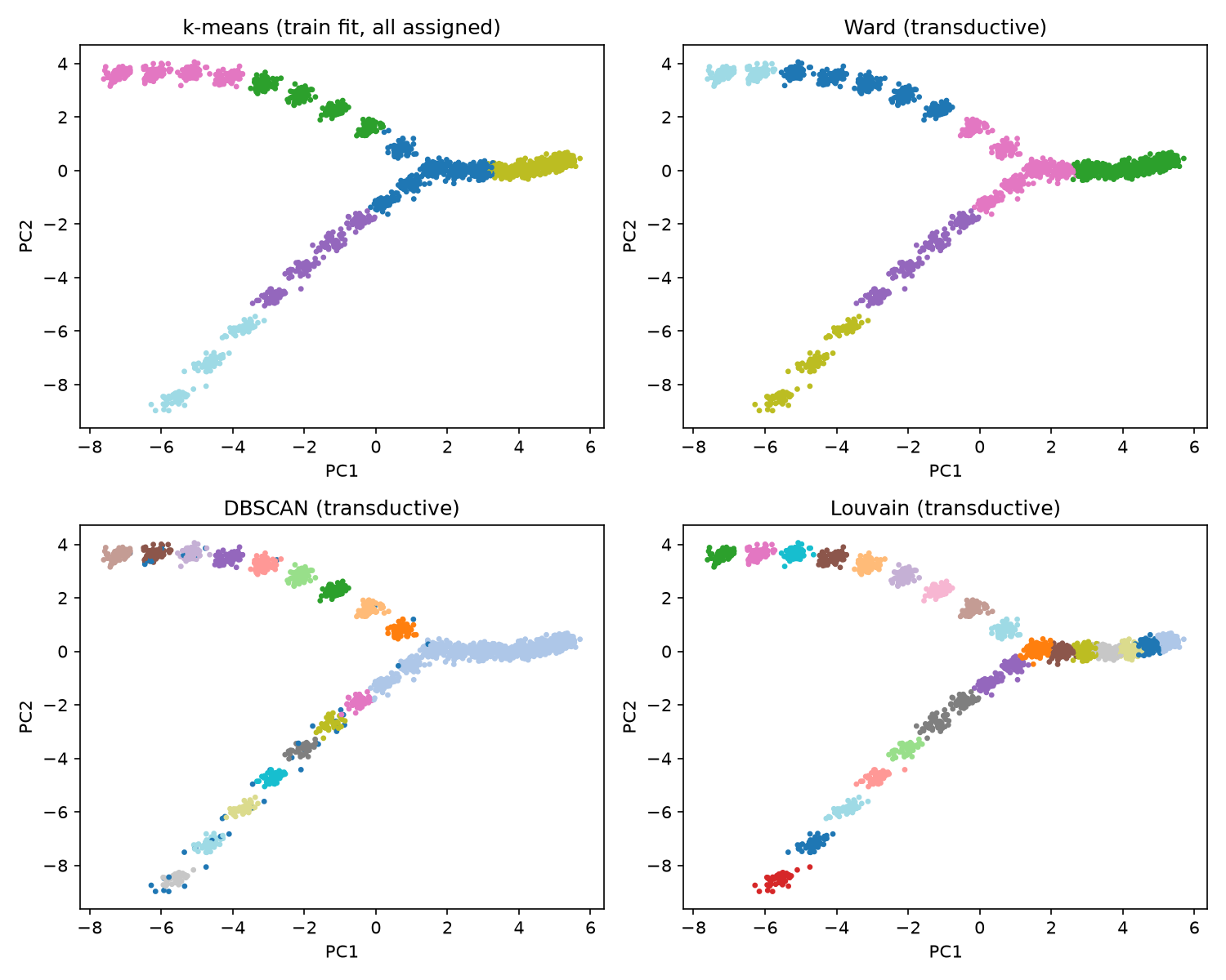
The scaler, PCA, and k-means centers use training sessions only. The script reports held-out distance to k-means centers as a geometric diagnostic. Ward, DBSCAN, and Louvain see all observations and are transductive. Their appealing plots are not held-out classification accuracy. Repeat the analysis across seeds, neighborhood sizes, and session-level resamples before interpreting a boundary.

6. Naming cell and narrative states

For cells, inspect marker expression, batch composition, and replication across donors before naming a cluster. A batch-specific group may represent a measurement process. A trajectory can also pass gradually between recognized cell types, making hard boundaries convenient approximations.

For character chat, sample conversation windows from each group and review them with a written annotation rubric. Names such as “trust building” or “conflict escalation” require evidence from the text. Speaker identity, language, or window length may explain a cluster instead. A label is not a diagnosis of a user’s internal psychology.

Use consented or synthetic conversations for teaching. Keep users or sessions together when splitting data, and avoid an encoder that reads future turns if the eventual task is online prediction.

7. Exercises with hints

1. Does a DBSCAN noise label mean a bad observation? No. It means the point did not fit the selected density criterion. Rare transitions may be scientifically useful; inspect them before removal.
2. If Louvain returns twice as many states at larger resolution, which result is correct? Neither follows from count alone. Compare stability, task usefulness, and independent annotations. Resolution changes the question.
3. Design a check for a “conflict” community. Blindly annotate sampled windows from that community and matched windows from others. Report agreement and confounding factors such as language or character. Do not choose examples only because they support the name.

Next, we turn these regions into possible paths and ask what additional assumptions are needed to call a path a trajectory.