A path fitted through observations is a geometric hypothesis about progression. To interpret it as development or story evolution, we must supply a root, validate its branches, and explain why the observations support that ordering. Snapshot geometry alone supplies neither a clock nor a causal direction.
Prerequisites: PCA, nearest-neighbor graphs, clustering, and shortest paths. 90 minutes: branching example 15, MST 15, principal curves and graphs 20, PAGA 15, lab and interpretation 25. By the end, you should distinguish a shortest tree from a fitted curve, a coarse connectivity graph, and a time series.
Start with the common setup. Download lesson07.py and the complete lab bundle.
1. One trunk, two possible continuations
Draw points along a horizontal trunk, then split them into an upper and a lower arm. Hide their collection order. A clustering algorithm gives regions, but the labels alone do not tell us which regions connect or where progression begins.
A useful initial answer is a tree through a small set of representative points. It exposes a candidate branch without pretending to recover each individual’s actual route. Add a loop to the drawing, however, and a tree must break it somewhere. Every method carries a topology assumption.
Our recurring project contains branching sessions observed at multiple steps. This lecture deliberately hides within-session transitions during fitting. We reconstruct a geometric baseline from observations, then use reserved sampling times to diagnose the result. Lecture 8 will exploit the actual sequence information.
2. Minimum spanning tree: a clear baseline
For representatives $\mu_1,\ldots,\mu_K$, let
$$w_{ab}=\|\mu_a-\mu_b\|_2.$$Among all trees connecting these vertices, choose
$$T^*=\arg\min_T\sum_{(a,b)\in T}w_{ab}.$$A tree has $K-1$ edges, no cycles, and one path between any two vertices. Kruskal’s algorithm sorts edges by increasing cost and adds an edge only if it does not create a cycle. This is a useful algorithmic link to an undergraduate graph course.
The weights here are distances, not affinities. Minimizing the sum of similarity weights would favor weak connections. If starting from a sparse neighborhood graph, use its edge lengths and recognize that disconnected components produce a forest, not a single spanning tree. SciPy’s graph routines provide both minimum spanning trees and shortest paths.
A tree over all noisy points can chase outliers. Our baseline first learns 14 k-means representatives from training sessions, then constructs a complete Euclidean graph between them. Completeness guarantees a tree, but can also force a connection across a gap. Inspect unusually long edges instead of interpreting them as proven transitions.
3. Principal curves and principal graphs
A principal curve replaces PCA’s straight line with a smooth curve through the middle of a distribution. Let $f(s)$ be a curve and $s_f(x)$ the parameter of the closest point on it. A classical principal curve satisfies the self-consistency condition
$$f(s)=\mathbb E[X\mid s_f(X)=s].$$An intuitive fitting procedure alternates projecting data onto a curve and smoothing the observations as a function of projection position. The smoothness choice prevents the curve from weaving through every noisy observation. Self-consistency does not guarantee that the curve is the true developmental trajectory, or that its solution is unique. See Hastie and Stuetzle’s original paper.
A single nonbranching curve cannot represent a Y-shaped lineage. Principal graphs extend the representation to vertices and edges with branch points. A teaching objective can combine distance to the graph with penalties:
$$\sum_i d(r_i,G)^2+\lambda\,\operatorname{length}(G)+\eta\,\operatorname{complexity}(G).$$This is a schematic objective, not one universal principal-graph algorithm. Real methods differ in elasticity, smoothness, topology changes, and regularization. Complexity control matters: adding enough branches always improves fit to noisy data. Our downloadable lab fits an MST baseline, not a principal-curve or elastic-graph implementation.
4. PAGA summarizes connectivity between groups
PAGA begins with a neighborhood graph of observations and a partition of its nodes. Each partition becomes a coarse node. Edge weights summarize evidence for connectivity between partitions relative to an appropriate random-connectivity expectation. Weak connections can then be filtered.
The crucial information comes from observed neighborhood edges between groups. It does not come from the distance between cluster centers alone. PAGA can retain disconnected structures and non-tree topology; an MST always imposes a tree when its input is connected. Calling a centroid MST “PAGA” would therefore change both the algorithm and its claims.
The PAGA paper explains the statistical connectivity construction and combines coarse paths with cell-level distance information. It is a tool for investigating topology, not proof that every retained edge is a biological lineage. Cluster resolution and neighbor construction still affect the result.
5. Pseudotime requires a root
Given a root $r$ and weighted graph $G$, a basic pseudotime is
$$\tau_i=d_G(r,i).$$The same undirected graph yields a different ordering when the root changes. An initial marker, known starting samples, or experimental design may justify a root. Choosing whichever root produces the expected answer and then claiming independent validation is circular.
Our lab projects each observation onto its nearest tree edge and measures distance from the selected root along that edge. This avoids giving every member of a cluster exactly the same value. The off-tree projection error remains a separate diagnostic.
Pseudotime is measured in embedding-distance units. Doubling a coordinate scale can change its values. A branch with greater distance need not take more minutes, and two branches at the same pseudotime need not be synchronized. A cell-cycle loop also cannot be represented faithfully by this tree coordinate.
6. Python and a root-change experiment
The following is the tree construction used by the complete script:
from common import make_dataset, prepare_embedding
from sklearn.cluster import KMeans
from scipy.spatial.distance import cdist
from scipy.sparse.csgraph import minimum_spanning_tree

data = make_dataset()
_, Z, _, _ = prepare_embedding(data, n_components=6)
km = KMeans(n_clusters=14, n_init=10, random_state=7).fit(Z[data["train"]])
centers = km.cluster_centers_
tree = minimum_spanning_tree(cdist(centers, centers))
print(tree.nnz, len(centers) - 1)
Run python lesson07.py --output outputs. The root is the representative nearest the mean of known initial training observations. The second panel uses the farthest tree vertex instead. Stars identify the respective roots.
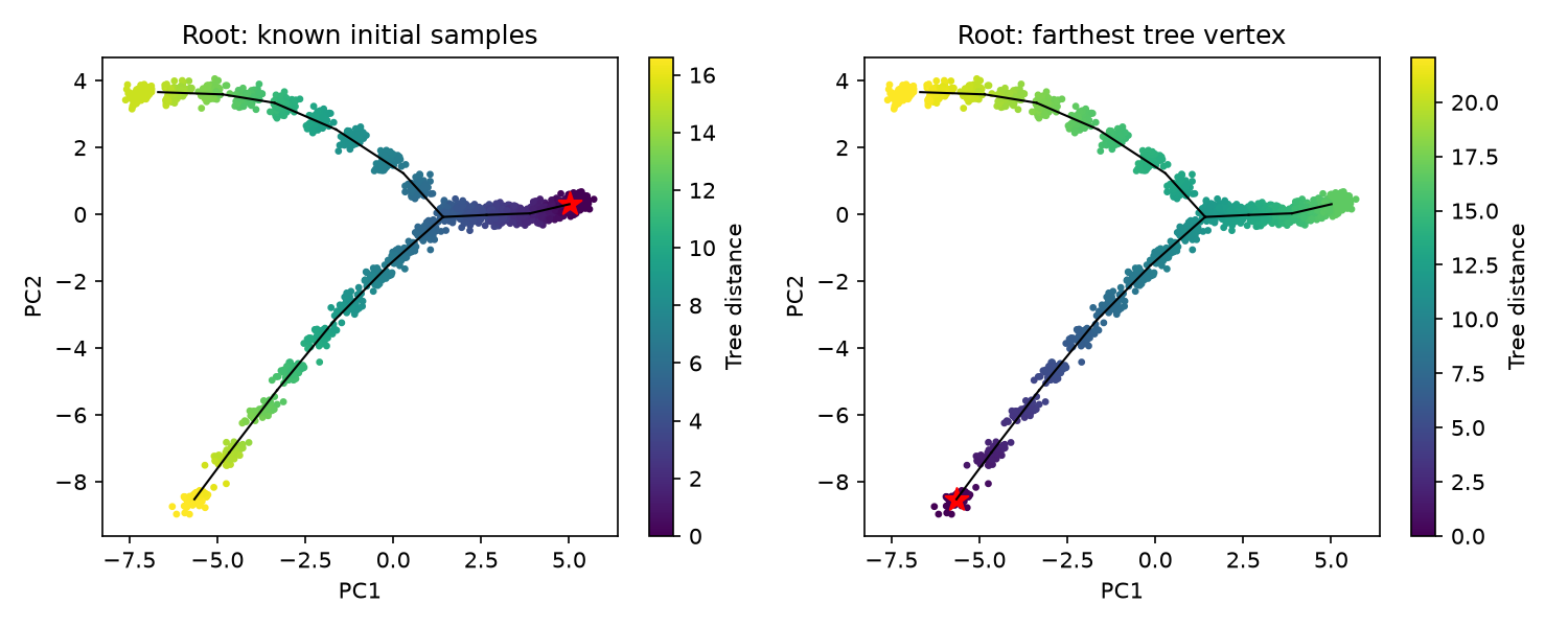
The script reports held-out projection error and Spearman correlation with observed sampling time, then repeats the correlation with the alternative root. All representation and tree fitting uses training sessions; held-out observations are projected afterward. This is a diagnostic of a fixed geometric reconstruction, not evidence of future forecasting or correct lineage ancestry. Hidden synthetic coordinates are not used for fitting.
7. Biological and narrative interpretation
For cells, use developmental markers and replicated samples to evaluate the trunk and branches. Destructive sequencing usually observes different cells at different stages, so proximity does not establish direct ancestry. Lineage tracing supplies a different kind of evidence.
For chat, branches could represent different continuations from similar story states. A branch that separates languages or characters may reflect the encoder rather than story evolution. Unlike many cell snapshots, ordered conversation turns are available; compare inferred paths with these actual within-session transitions. Use only windows available at the analysis time when developing an online application.
8. Exercises with answers
- Why does using affinity in a minimum spanning tree reverse the intended preference? Small similarity means dissimilarity, but the optimizer chooses small weights. Supply lengths or a justified cost transformation.
- Can high correlation with collection time prove the branches are correct? No. One ordering can correlate strongly with time while joining incorrect endpoints. Evaluate topology and domain evidence separately.
- What should happen to a loop? A tree breaks at least one connection. Compare a method allowing cycles, and report the tree assumption rather than interpreting the cut as a discovered biological event.
Next, observed sequences will let us estimate transition probabilities instead of deriving order solely from geometry.