Trajectory ML 8: Markov Models, HMMs, and State Space Models

Observed order lets us ask a stronger question than geometric proximity: given the current state, what happens next? A Markov model answers with a transition table. An HMM additionally recognizes that our state labels are uncertain. A state space model lets the hidden state vary continuously.

Prerequisites: conditional probability, matrix multiplication, clustering, and dynamic programming. 90 minutes: sequence example 10, Markov estimation 15, HMM inference 30, lab 20, continuous states and applications 15. The learning target is to compute transitions without crossing session boundaries and explain which observations an inference method is allowed to use.

Use the shared environment, lesson08.py, and complete lab bundle.

1. Two short sequences are not one long sequence

Suppose two sessions have discrete states A, A, B and C, C. We observed A→A, A→B, and C→C. We did not observe B→C. Concatenating the rows and counting every adjacent pair creates a transition that never happened.

In a 2D toy plot, place A, B, C at three locations and draw the measured arrows. Distances do not determine their direction or probability. Two nearby states might rarely follow one another, while a larger jump may occur frequently. This differs fundamentally from Lecture 5’s similarity-based random walk.

The first-order Markov assumption is

It is a model assumption, not something guaranteed by dimensionality reduction. A state representation must retain enough relevant history for the approximation to be useful. Conversation topics and unresolved promises often violate a memoryless model.

2. Estimate a transition matrix

Let $N_{ij}$ count state $i$ followed by state $j$ within training sessions. With $K$ states and symmetric pseudocount $a>0$,

Smoothing avoids assigning zero probability to a transition merely because a small sample did not contain it. It does not prove the transition is physically possible. Known forbidden transitions require an explicit structural model.

Rows sum to one. A row distribution $p_t$ evolves as $p_{t+1}=p_tA$. Under a time-homogeneous model, $A^h$ gives transitions over $h$ equal steps. A chat turn and an hour are different units; irregular gaps need additional modeling rather than pretending they are equal.

Our lab fits k-means on training observations, assigns all observations to those centers, and estimates transitions between the resulting labels. The labels are a learned discretization, not known ground-truth states.

3. HMM: states generate uncertain observations

Let the hidden state be $s_t\in\{1,\ldots,K\}$ and the observed PCA vector be $r_t$. An HMM combines an initial distribution $\pi$, a transition matrix $A$, and emission densities $b_j(r)=p(r\mid s=j)$:

The model assumes the observation depends on the current hidden state, and is conditionally independent of other observations given that state. Gaussian emissions are a convenient baseline for continuous coordinates. A Gaussian density is not a discrete probability and may exceed one.

There are three separate tasks: evaluate how well a sequence fits a fixed model, infer its states, and learn model parameters. Rabiner’s original tutorial organizes the classical HMM algorithms around these tasks.

4. Forward, backward, and Viterbi

Forward inference sums over all possible histories ending in a state. Define $\alpha_t(j)=p(r_{1:t},s_t=j)$. Then

The sequence likelihood is $\sum_j\alpha_T(j)$. Dynamic programming reduces exponentially many state sequences to $O(TK^2)$ work for dense transitions. Normalize at each step or calculate in log space to avoid underflow.

Backward inference summarizes the remaining observations: $\beta_t(i)=p(r_{t+1:T}\mid s_t=i)$, with

The smoothed state probability is proportional to $\alpha_t(i)\beta_t(i)$. It uses observations after time $t$. In contrast, normalizing $\alpha_t$ gives the filtered distribution using only observations available so far. Using a smoothed state as an online forecast feature leaks future information.

Viterbi asks for the single most probable whole path, rather than the marginal winner at every time. In log space,

Store the maximizing predecessor, then backtrack from the final winner. Replacing the maximum with logsumexp gives the forward update. These two operations answer different questions, so the Viterbi path and pointwise posterior winners can disagree. The Stanford HMM chapter provides a complementary dynamic-programming treatment.

5. Python: transparent inference, honest fitting

The downloadable script implements log-space forward/backward and Viterbi directly. Its transition-counting function uses next_index to preserve boundaries:

from common import make_dataset, prepare_embedding
from sklearn.cluster import KMeans
from lesson08 import estimate_transitions

data = make_dataset()
_, Z, _, _ = prepare_embedding(data, n_components=6)
km = KMeans(n_clusters=6, n_init=10, random_state=7).fit(Z[data["train"]])
labels = km.predict(Z)
A = estimate_transitions(labels, data["next_index"], data["train"], 6)
print(A, A.sum(axis=1))

Run python lesson08.py --output outputs. The complete script initializes diagonal Gaussian emissions from training-cluster means and variances, and the initial-state distribution from training-session starts. It does not run Baum–Welch. Baum–Welch is EM: infer expected state and transition counts, then update parameters and repeat. That is a useful extension, but should not be claimed for this baseline.

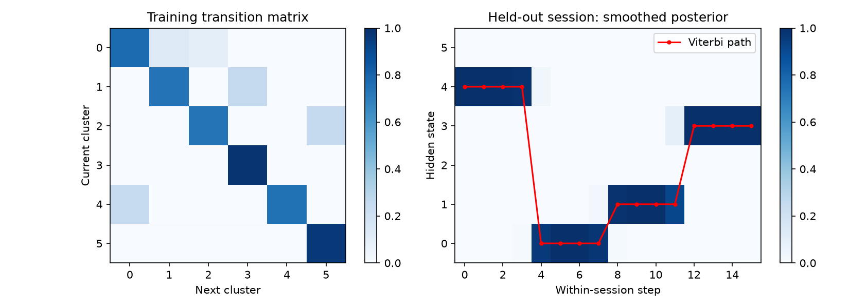
The transition metric is held-out next-cluster negative log-likelihood, compared with a training marginal-frequency baseline. The HMM metric is observation log density per step. They evaluate different predictions and cannot be compared numerically as one score. The posterior plot uses smoothing on a complete held-out session; it is retrospective inference. Whole-session splitting prevents training on later turns of an evaluated session.

6. Continuous state space models

A continuous hidden vector can change without jumping between categories. A linear Gaussian model is

With a Gaussian initial state and independent Gaussian noises, the Kalman filter recursively predicts a mean and covariance, then corrects them using the new observation. If the predicted state mean is $m_t^-$, the update has the form

The Kalman gain $K_t$ depends on uncertainty. A noisy observation receives less weight; a highly uncertain prediction receives a larger correction. Kalman’s original paper develops this recursive filtering view. General nonlinear state space models require different or approximate inference; not every model bearing “SSM” in its name uses a Kalman filter.

7. Cells, narratives, and exercises

For biology, repeated observations of tracked cells can support transition estimation. Unpaired cells from successive collection times do not provide individual transitions for free. For narrative analysis, turns are paired within sessions, but turn length, speaker, prompts, and interventions can change transition probabilities. Predictive association with these factors is not a causal effect.

1. Count A,A,B and C,C without smoothing. A has probabilities 1/2 to A and B; C goes to C. B has no outgoing observation, so its row cannot be estimated from these data alone.
2. Why not multiply raw probabilities for a thousand steps? Products can underflow. Use scaled forward messages or log probabilities and logsumexp.
3. Can an online system use the displayed smoothed posterior? Not at an intermediate turn, because the backward message reads future observations. Use filtering, and evaluate only information available at the prediction time.

We now have actual transition evidence. Next, we will ask how large each movement is and learn a vector field.