Trajectory ML 09: Learn where a state moves next

A trajectory tells us where a system has been. A vector field tells us which direction it tends to move from its current state. This distinction turns our geometric map into a forecasting model. It also exposes a limitation: arrows are only as meaningful as their coordinates and the evidence used to estimate them.

Preparation and plan. Review PCA, regression, Markov models, and a derivative. Allow 90 minutes: 15 for finite differences, 20 for fields and RNA kinetics, 35 for the Python lab, and 20 for error analysis. After this lesson you should be able to construct legal adjacent pairs, compare one-step and free-rollout predictions, and explain why an RNA-velocity arrow differs from a measured chat transition. Use the shared setup, complete lab, or all labs.

First measure one movement

Imagine a chat state with horizontal coordinate “plot progress” and vertical coordinate “tension.” At time 2 it is at $(1,0)$; at time 2.5 it is at $(1.2,0.3)$. The displacement is $(0.2,0.3)$, but the average velocity is $(0.4,0.6)$ per time unit. Dividing by elapsed time makes observations with different gaps comparable.

For paired states, define

This approaches a derivative only under suitable smoothness and sufficiently short intervals. For chats, a turn is also a defensible time unit. A turn-based velocity and a per-minute velocity answer different questions; an overnight pause should not silently become one ordinary step.

A branch creates an additional problem. The same location might precede an upward or downward move. A squared-error regressor averages these moves, possibly pointing into an empty region between branches. More data alone cannot restore information discarded by the state representation. Add history or relevant context, or predict a distribution over next states.

From arrows to a function

We fit a rule that generalizes from observed arrows:

Time is included in this lab because the synthetic process need not be autonomous. If a model only takes $z$, it assumes the same state has the same expected velocity regardless of when it is reached. This is a modeling decision, not a consequence of drawing a scatterplot.

Our baseline averages velocities among 40 neighboring training inputs. It is easy to inspect and introduces useful smoothing. A neural network could replace it, but should first beat simple baselines on sessions it has never seen.

Finite differences amplify observation noise. If two independent scalar measurements have noise variance $\sigma^2$, their difference divided by $\Delta t$ has variance $2\sigma^2/\Delta t^2$. Tiny sampling intervals therefore do not automatically produce reliable derivative estimates. Smooth trajectories, repeat measurements, and model uncertainty when appropriate; never smooth across session boundaries.

The lab: lawful pairs, honest forecasts

The dataset contains 120 synthetic sessions and a fixed observation window. We first learn scaling and PCA from training sessions. The following excerpt is the pairing and regression core of the downloadable script:

import numpy as np
from sklearn.neighbors import KNeighborsRegressor
from common import make_dataset, prepare_embedding

data = make_dataset()
_, Z, _, _ = prepare_embedding(data)
current = np.flatnonzero(data["next_index"] >= 0)
following = data["next_index"][current]
dt = data["time"][following] - data["time"][current]
velocity = (Z[following] - Z[current]) / dt[:, None]
features = np.column_stack([Z[current], data["time"][current]])
fit = data["train"][current]
model = KNeighborsRegressor(n_neighbors=40, weights="uniform")
model.fit(features[fit], velocity[fit])
predicted = Z[current[~fit]] + dt[~fit, None] * model.predict(features[~fit])

Run python lesson09.py --output outputs from the extracted lab directory. The complete script asserts positive gaps and matching session IDs, then saves the figure below. z_true is never a training feature. Pairing consecutive rows without checking session identity would fabricate a transition from one person’s ending to another person’s beginning.

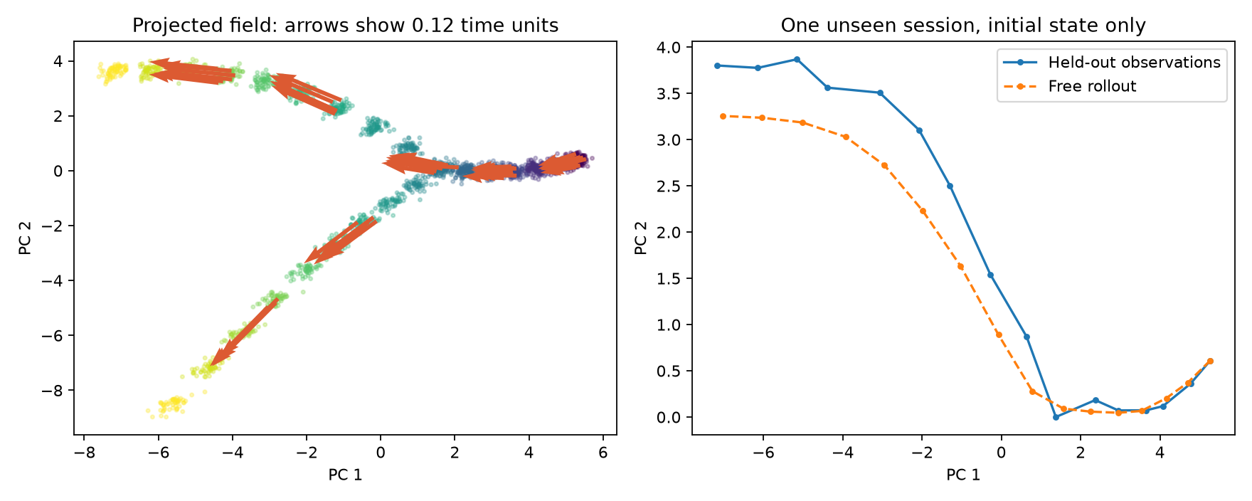
The left panel shows projected velocities scaled to 0.12 time units. The right panel begins with a real held-out initial state, then repeatedly feeds predictions back into the model:

One-step evaluation instead supplies the actual state at every step, a teacher-forcing-style evaluation. It measures local accuracy without the accumulated errors of a free rollout. In the supplied seeded run, one-step MSE is about 0.035, compared with 0.516 for persistence. Rollout MSE rises to about 7.51, although staying forever at the initial state is worse at 26.74. These are coordinate-dependent toy errors, not biological performance estimates. Report both tasks because deployment may require the harder one.

What RNA velocity adds

A typical single-cell RNA-sequencing experiment destroys the measured cell. We therefore cannot simply subtract its expression tomorrow from its expression today. RNA velocity instead uses molecular information about unspliced and spliced RNA to estimate a local expression derivative. The original work establishes this idea; its supplementary material also discusses estimation and visualization limitations. La Manno et al., 2018

A simplified kinetic model for one gene is

Here $u$ is unspliced abundance, $s$ is spliced abundance, and $\alpha,\beta,\gamma$ describe transcription, splicing, and degradation. With $u=4$, $s=3$, $\beta=1$, and $\gamma=1$, the predicted spliced derivative is $1$. It is an inference from a kinetic model, not an observed next cell.

Steady-state assumptions and rate assumptions can fail. scVelo extends the modeling to transient states with dynamical kinetics; it does not make uncertainty or model misspecification disappear. Bergen et al., 2020

For chats we often possess ordered observations directly, but embeddings still depend on the encoder, window length, speaker, and prompt. A moving average window can produce apparently smooth movement even when the underlying interaction changes abruptly. The script estimates narrative-feature movement only; it does not estimate RNA velocity.

Coordinates limit the claim

For a fixed linear projection $z=W^\top x$, a velocity projects as $v_z=W^\top v_x$. For a differentiable nonlinear encoder $z=g(x)$, the corresponding local rule is $v_z=J_g(x)v_x$. Simply moving arrows onto a UMAP picture is not generally this calculation.

A hidden direction can disappear in two dimensions; a distorted embedding can change apparent speed. Treat the figure as a model diagnostic, then validate in the space relevant to the scientific question. Perturbing a state and observing its response is a separate causal problem, reserved for lesson 12.

Exercises

1. Change units. A displacement is $(2,-1)$ over four turns. What is the velocity? Answer: $(0.5,-0.25)$ per turn. If each turn lasts a different duration, there is no unique conversion to per-minute velocity without timestamps.
2. Break the evaluation deliberately. Replace free-rollout inputs by each true held-out state. Why does error usually drop? Hint: the model no longer has to survive its own accumulated errors; this is a different prediction task.
3. Test missing memory. Construct two sessions that cross the same 2D point with opposite outgoing directions. Fit a local regressor there. Expected finding: the average arrow can be nearly zero despite both sessions moving. Add previous velocity to the input and compare on new sessions.

You now have a local rule for moving a state. The next lesson asks what is identifiable when only whole populations are observed at each time.