When individuals cannot be followed, we can still compare populations. Optimal transport (OT) asks how to redistribute one population into another while paying as little movement cost as possible. The result is a coupling consistent with specified constraints. It is not a recovered list of who actually became whom.
Preparation and plan. Review probability distributions, matrices, distances, and the PCA state space. Use 90 minutes: 15 for the matching puzzle, 25 for constraints and entropy, 30 for Python, and 20 for interpretation. You should leave able to write the balanced OT problem, verify its marginal constraints, and explain the effect of regularization. Start with the shared environment, complete script, and lab archive. This lesson adds the POT package, imported as ot.
Two snapshots, no identity labels
At an early time, three cells are near the center of a state map. Later, two groups appear on opposite branches. The measurements came from different cells. Nearest-neighbor matching sounds tempting, but it can send all early mass to the same convenient destination and ignore the rest of the observed later population.
Use a smaller example first. Put two source points at $(0,0)$ and $(1,0)$ and two target points at $(0,1)$ and $(1,1)$. Give each point mass $1/2$. With squared Euclidean cost, vertical moves cost 1 while crossed moves cost 2. The cheapest coupling sends half the mass vertically from each source. Its total cost is 1, not 2: each move carries only half the population.
If both targets instead lie at the same location, multiple identities may be equally compatible with the data. A solver cannot create evidence that was never measured. This ambiguity persists in larger, more attractive visualizations.
The missing ingredient is conservation
Let source masses be $a_i$, target masses $b_j$, with both summing to 1. Define $\gamma_{ij}$ as the amount of mass sent from source $i$ to target $j$. Balanced transport solves
$$ \min_{\gamma\geq0}\sum_{i,j}C_{ij}\gamma_{ij},\qquad \gamma\mathbf 1=a,\quad \gamma^\top\mathbf 1=b. $$The row constraint says each source sends exactly its available mass. The column constraint says each destination receives its required mass. A coupling has entries for every source-target pair; it need not be a permutation or a one-to-one assignment.
This distinction allows unequal sample counts. Fifty observations and eighty observations can each represent total probability 1, assigning weights $1/50$ and $1/80$. Equal total mass does not mean equal numbers of cells or sessions in the real world. Normalization discards absolute abundance information.
The cost encodes our scientific preference. Euclidean cost rewards short straight paths in the chosen representation. A geodesic cost can penalize crossing gaps, but then the neighborhood graph becomes an additional assumption. Feature scaling, batch effects, and missing states all influence what “cheap” means.
Which quantity is Wasserstein distance?
For a metric $d$ and exponent $p\geq1$,
$$ W_p(\mu,\nu)=\left[\min_{\gamma\in\Pi(a,b)} \sum_{ij}d(x_i,y_j)^p\gamma_{ij}\right]^{1/p}. $$If $C_{ij}=\|x_i-y_j\|^2$, the unregularized optimal cost is $W_2^2$; take its square root to report $W_2$. If $C=d$, the optimal cost is $W_1$. Calling any transport objective “Wasserstein distance” loses both the exponent and the assumptions that make it a metric.
The lab reports exact $W_2$ using a small linear-programming problem. It separately reports the movement cost of entropy-regularized plans. Those are distinct outputs, even when their values are close.
Entropy spreads mass and speeds computation
Add a regularizer:
$$ \min_{\gamma\in\Pi(a,b)}\langle C,\gamma\rangle +\varepsilon\sum_{ij}\gamma_{ij}(\log\gamma_{ij}-1). $$Increasing $\varepsilon$ rewards a more diffuse plan. Decreasing it emphasizes low movement cost but can make numerical optimization harder. Its units must match the cost, so a value such as 0.2 is meaningless without the cost scale.
Writing $K_{ij}=\exp(-C_{ij}/\varepsilon)$, Sinkhorn scaling alternates
$$ \nu\leftarrow a/(K\omega),\qquad \omega\leftarrow b/(K^\top\nu),\qquad \gamma=\operatorname{diag}(\nu)K\operatorname{diag}(\omega), $$where division is elementwise. Alternating row and column scaling enforces the two marginals. Stable log-domain implementations avoid explicitly underflowing tiny kernel entries. Entropic transport and this computational connection are developed in Cuturi, 2013.
Regularized OT is generally biased as a distribution discrepancy: transporting a distribution to itself can have a nonzero regularized value. A debiased Sinkhorn divergence is a separate construction. We do not compute one in this lab.
Python: inspect conservation before the picture
The full script builds early and late snapshots from disjoint training-session sets, intentionally withholding individual correspondence. PCA is fitted on training sessions. With arrays A and B holding these projected snapshots, the transport core is:
import numpy as np
import ot
from common import make_dataset, prepare_embedding
from lesson10 import population_snapshots

data = make_dataset()
_, Z, _, _ = prepare_embedding(data)
A, B = population_snapshots(data, Z)
a = np.full(len(A), 1 / len(A))
b = np.full(len(B), 1 / len(B))
cost = ot.dist(A, B, metric="sqeuclidean")
exact_plan = ot.emd(a, b, cost)
exact_w2 = np.sqrt(np.sum(exact_plan * cost))
normalized_cost = cost / np.median(cost)
plan = ot.sinkhorn(a, b, normalized_cost, reg=.2,
                   method="sinkhorn_log", numItermax=5000,
                   stopThr=1e-10)
assert np.max(abs(plan.sum(axis=1) - a)) < 1e-6
assert np.max(abs(plan.sum(axis=0) - b)) < 1e-6
Run python lesson10.py --output outputs after the shared setup. The documented POT APIs expose both unregularized and regularized solvers. POT documentation
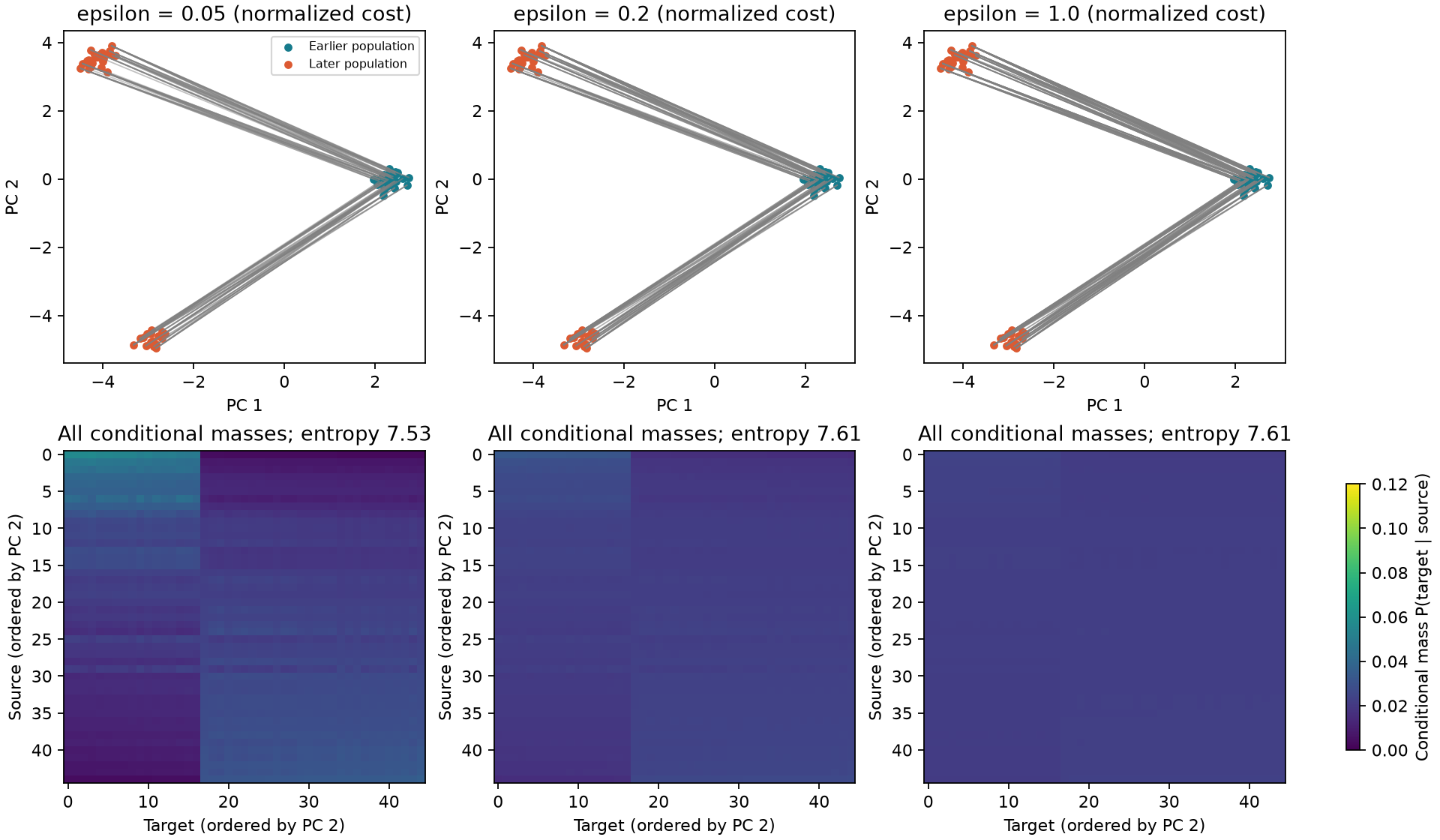
The seeded run gives exact $W_2$ around 7.14 in PCA coordinate units. The script tests $\varepsilon=0.05,0.2,1$ after dividing the cost by its median. Marginal residuals must remain below $10^{-6}$. The top panels show the two largest connections per source. The bottom heatmaps show every conditional mass, with both axes ordered by PC 2 and a shared color scale. The numerical conservation check uses the entire matrix.
Larger entropy usually spreads visible connections. A dense diagram does not mean the model discovered more biological transitions. It means the chosen optimization preference distributes uncertainty differently.
Biological and narrative interpretations
Cell populations grow, divide, and die. A balanced normalized coupling can describe distributional shape changes while hiding growth. Unbalanced OT relaxes conservation through penalties or explicit growth models. Waddington-OT illustrates how transport ideas can contribute to developmental analysis across sampled populations. Schiebinger et al., 2019
For character chat, compare state distributions at early and late turns or across cohorts. A change may reflect progression, user selection, censoring, or a different mixture of characters. If session identities are available, evaluate the inferred coupling against real transitions rather than discarding this extra evidence. Couplings across product versions do not by themselves identify a prompt’s causal effect.
Exercises
- Check a plan. For $a=b=(1/2,1/2)$, is $\gamma=\left[\begin{smallmatrix}.5&0\\.5&0\end{smallmatrix}\right]$ legal? Answer: rows are correct; columns are $(1,0)$, so it violates the target marginal.
- Check the root. A squared-distance OT objective is 9. What is $W_2$? Answer: 3. A regularized plan with movement cost 9 does not necessarily attain the unregularized optimum.
- Change the geometry. Multiply one feature by 10, rebuild costs, and compare plans. Hint: squared distances multiply that feature’s contribution by 100. Explain why preprocessing is part of the transport model, not just a cosmetic choice.
We have described a coupling between populations. Next we learn a continuous vector field that moves a whole distribution between endpoints.