A neural network can predict a velocity, and a numerical solver can repeatedly use that velocity to move a state. This is the central idea behind a Neural ODE. The same machinery can also move an entire probability distribution. What the motion means depends on the supervision: observed time and an artificial generation clock are not interchangeable.
Preparation and plan. Review derivatives, neural-network regression, lesson 9’s vector field, and lesson 10’s coupling. Allow 100 minutes: 20 for ODEs, 15 for stochasticity and density, 35 for flow matching and Python, and 30 for diagnostics. The target is an executable 2D generative model and a precise statement of what it does not identify. Use the setup guide, complete PyTorch lab, or all labs.
A small step is a residual update
Start at $(0,0)$ with constant velocity $(1,2)$. With step size $h=0.1$, ten updates $z\leftarrow z+h(1,2)$ reach $(1,2)$. For a learned field, the update becomes
$$ z_{k+1}=z_k+h f_\theta(z_k,t_k). $$This is the explicit Euler method. An ODE describes the continuous model that these discrete steps approximate:
$$ \frac{dz}{dt}=f_\theta(z,t),\qquad z(t_1)=z(t_0)+\int_{t_0}^{t_1}f_\theta(z(t),t)\,dt. $$The network specifies the derivative; the solver evaluates the path. A smaller step can reduce numerical error, but it cannot repair an incorrect learned field. Adaptive solvers adjust their work to a requested tolerance, and stiff fields may still be expensive. Neural ODEs make this separation between parameterized dynamics and numerical integration explicit. Chen et al., 2018
Under regularity conditions giving uniqueness, exactly the same initial state follows exactly one deterministic ODE path. A distributed set of initial states can end in two modes, but that is not stochastic branching of one identical state. To represent multiple futures from identical observed evidence, include uncertain latent initial conditions, conditioning information, or stochastic dynamics.
Noise changes the model, not only the picture
An Itô SDE can be written as
$$ dz=f_\theta(z,t)\,dt+\Sigma(z,t)\,dW_t. $$The drift $f_\theta$ controls average local movement; the diffusion matrix $\Sigma$ controls random fluctuations. $W_t$ is Brownian motion. Its increments over a step $h$ have variance proportional to $h$, so Euler–Maruyama uses
$$ z_{k+1}=z_k+h f_\theta(z_k,t_k)+\sqrt h\,\Sigma(z_k,t_k)\xi_k, \qquad \xi_k\sim\mathcal N(0,I). $$The $\sqrt h$ matters. Using $h\xi_k$ instead changes the noise behavior as the step size shrinks. Itô and Stratonovich conventions can imply different drifts for state-dependent noise; this lesson uses Itô and implements only the deterministic case.
A flow also transports density
An invertible map $y=g(x)$ changes density according to
$$ \log p_Y(y)=\log p_X(x)-\log|\det J_g(x)|. $$This is the basic change-of-variables view of a normalizing flow. For a sufficiently regular continuous flow, its local counterpart is
$$ \frac{d}{dt}\log p_t(z(t))=-\nabla\!\cdot f_\theta(z(t),t). $$A field that expands volume lowers density along the flow. This explains why trajectories and distribution modeling can share machinery. Our lab learns velocities without evaluating likelihood or the divergence, so it should not report a likelihood score merely because the architecture defines a flow.
Flow matching makes a supervised regression problem
Pick an early point $x_0$ and a late point $x_1$. For a randomly sampled artificial time $t\in[0,1]$, construct
$$ x_t=(1-t)x_0+tx_1,\qquad u_t=x_1-x_0. $$The straight segment provides both a training input and its exact conditional velocity. Fit
$$ \mathcal L(\theta)=\mathbb E_{x_0,x_1,t} \left\|f_\theta(x_t,t)-(x_1-x_0)\right\|_2^2. $$Different endpoint pairs can pass near the same $(x_t,t)$ with different velocities. Squared-error regression learns their conditional average. The population field obtained in the ideal limit transports the chosen probability path under suitable assumptions. Finite data, finite network capacity, and imperfect optimization introduce error. Conditional flow matching provides a practical way to train such fields without solving an ODE inside each training step. Lipman et al., 2022
The coupling is a modeling choice. This lab draws endpoints independently. It does not use OT pairs and does not recover the hidden identity of a session. Training straight conditional segments also does not imply that every generated path will be straight.
Python: train a field and integrate it
The complete lab uses the same synthetic observations as earlier lessons. PCA and additional coordinate standardization are fitted on training sessions. Early frames ($t_{\mathrm{obs}}\leq0.15$) supply the source population; late frames ($t_{\mathrm{obs}}\geq0.85$) supply the target. The network has two hidden layers with 64 units and receives two state coordinates plus interpolation time.
This copy-and-run entry point executes all preparation, 700 minibatch updates, Euler integration, and diagnostics from the downloadable implementation:
from pathlib import Path
from lesson11 import run

metrics = run(Path("outputs"))
print(metrics["endpoint_sliced_w1"])
print(metrics["euler_refinement_rmse"])
The script can also be run as python lesson11.py --output outputs. Its training loop samples 128 pairs, builds the convex interpolation, evaluates velocity MSE, and applies Adam. It intentionally uses a small CPU model suitable for inspection.
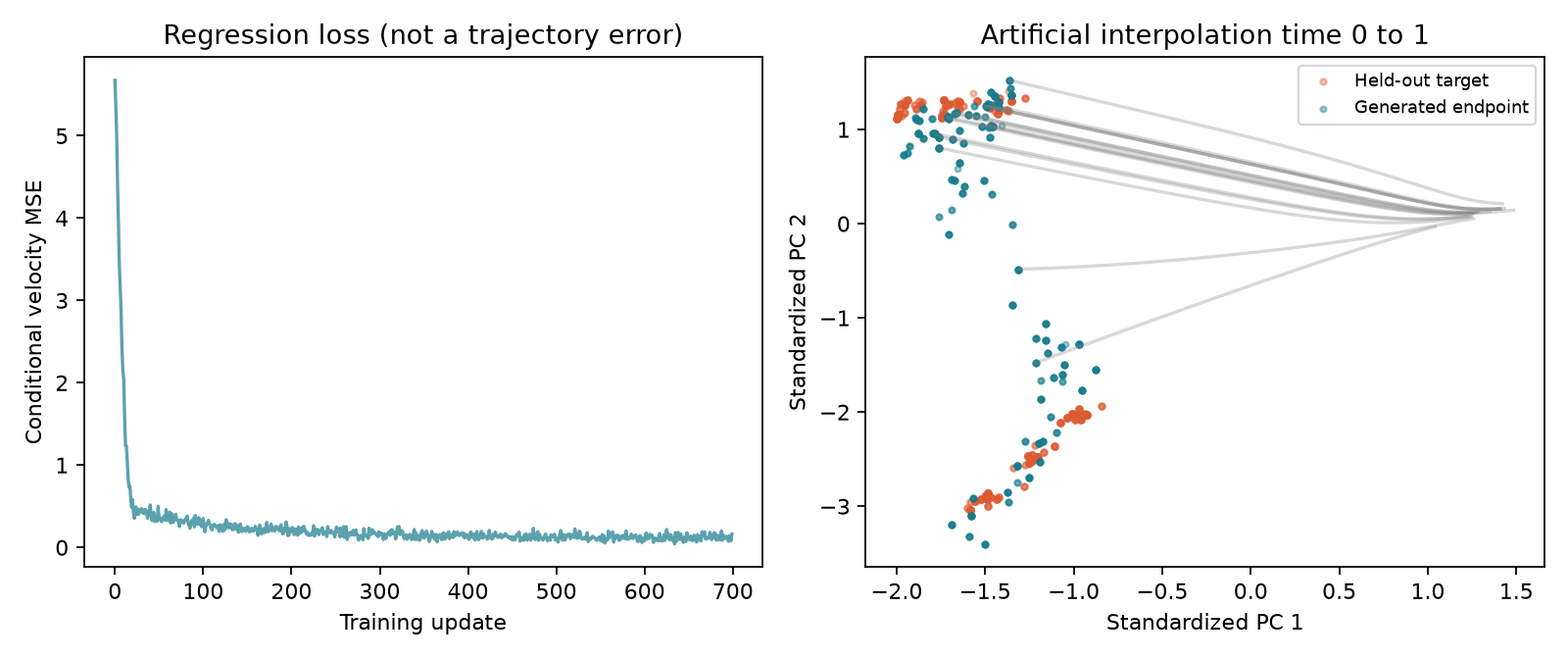
Testing starts from samples belonging to held-out sessions and compares generated endpoints with held-out late states. A sliced $W_1$ diagnostic projects both populations onto 64 directions, sorts each projection, and averages absolute quantile differences. It is a distribution comparison, not a paired trajectory error.
In the seeded run, this diagnostic drops from about 2.17 before transport to 0.45 after transport. Integrating with 80 versus 160 Euler steps changes paired generated endpoints by an RMSE around 0.024. The latter checks numerical sensitivity, while the former checks population matching. Neither demonstrates correct biological dynamics. A low training loss alone establishes even less.
The biological clock is a separate claim
A model fitted to real repeated observations can attempt to predict actual temporal dynamics. It still needs appropriate state variables, temporal validation, and uncertainty analysis. Our generative model sees endpoint populations and an invented interpolation. Many different intermediate paths could fit those same endpoints.
In biology, smooth generated paths may support hypotheses about population movement, but intermediate-time measurements and perturbations are needed to test them. In character chat, a path between “introduction” and “resolution” embeddings may visit regions no real conversation can reach. Decoding, coherence constraints, and held-out actual sessions provide additional checks; they do not appear automatically from endpoint matching.
A Schrödinger bridge adds a reference stochastic process and seeks a path distribution connecting endpoint marginals while staying close to that reference in relative entropy. It connects stochastic control and transport, but is not another name for this independent-pair flow-matching lab. De Bortoli et al., 2021
Exercises
- Separate errors. Halve Euler’s step size without retraining. Which error can improve? Answer: integration error. Representation, estimation, and endpoint-only identifiability problems remain.
- Check the noise scale. For scalar diffusion $\sigma=2$ and $h=0.01$, what is the noise standard deviation per step? Answer: $\sigma\sqrt h=0.2$, not $0.02$.
- Test what was learned. Compare generated paths with true held-out intermediate observations, which the training objective never used. Hint: endpoint distribution agreement can coexist with poor temporal paths. Label interpolation time separately from observation time in your report.
We can now describe and generate movement. The final lesson asks how to evaluate outcomes and when changing an input supports a causal claim.