A state associated with dropout is not necessarily a state that causes dropout. This final lesson separates three useful questions: when an event occurs, which outcome is likely, and what an intervention changes. They require different labels, assumptions, and evaluation.
Preparation and plan. Review conditional probability, logistic regression, train/test splitting, and the series’ state representation. Allow 110 minutes: 25 for survival, 25 for fate prediction, 35 for causal reasoning and the lab, and 25 for project design. Use the setup guide, complete script, and lab archive. Additional packages are pandas and lifelines.
The event may not have happened yet
Four sessions have follow-up records: an event at time 2, observation ending without an event at 3, an event at 4, and observation ending without an event at 5. The second record does not mean “survived forever” or “dropped out at 3.” We know only that its event time exceeds 3. This is right censoring.
Write the event time as $T$, censoring time as $C$, and observed record as
$$ U=\min(T,C),\qquad \delta=\mathbf 1[T\leq C]. $$The survival function is $S(t)=P(T>t)$. At distinct event times $t_j$, the Kaplan–Meier estimator uses event counts $d_j$ and the number still at risk immediately before that time, $n_j$:
$$ \widehat S(t)=\prod_{t_j\leq t}\left(1-\frac{d_j}{n_j}\right). $$In our four-record example, survival becomes $3/4$ at time 2. Censoring at 3 removes one record from later risk sets without lowering the curve. At time 4, two remain at risk, so survival becomes $(3/4)(1/2)=3/8$. The final censored record does not force survival to zero. For this unadjusted Kaplan–Meier curve, censoring must be independent of event time in the population being summarized. Conditional independence can justify appropriately adjusted survival models, but does not by itself justify a pooled, unadjusted curve. Informative loss to follow-up needs additional methods. Kaplan–Meier implementation and examples
A hazard is not always a probability
For discrete turns, a hazard can be the probability
$$ h_k=P(T=k\mid T\geq k). $$For continuous time, use a rate:
$$ \lambda(t)=\lim_{\Delta t\downarrow0} \frac{P(t\leq TCox proportional hazards relates covariates $q$ to this rate:
$$ \lambda(t\mid q)=\lambda_0(t)\exp(\beta^\top q). $$For one additional unit of a covariate, $e^{\beta_j}$ is a hazard ratio under the model, not a ratio of event probabilities. Ignoring ties, its partial likelihood compares each observed event with its contemporaneous risk set:
$$ L(\beta)=\prod_{i:\delta_i=1} \frac{e^{\beta^\top q_i}}{\sum_{j\in R(U_i)}e^{\beta^\top q_j}}. $$The baseline hazard cancels in this comparison. Proportionality, covariate specification, and censoring assumptions still matter; a fitted coefficient is not automatically causal. Cox fitting and diagnostics
Fate prediction has a prediction time
Place each session on our 2D state map at an early landmark. Color it by its eventual branch. We want
$$ P(Y=k\mid\text{information available by the landmark}). $$A prediction cannot use a final summary, later turns, or a trajectory feature calculated from its future. Even an unsupervised scaler or PCA should be fitted within the permitted training data. The lab fits both transformations on training-session frames with observation time at most 0.4, averages these prefix coordinates into one row per session, and fits logistic regression to final branch labels.
The simulator deliberately provides no intended branch signal before branching. Accordingly, the held-out result is poor: AUC about 0.415, Brier score 0.288, versus 0.251 for a constant training-prevalence predictor. Lower Brier is better. This is evidence that the early representation does not support the requested prediction, not an invitation to smuggle future observations into the features.
AUC assesses ranking. Brier score and log loss assess probabilistic predictions. A calibration plot compares predicted probabilities with observed frequencies, but four bins from only 30 test sessions cannot establish reliable calibration. In real data, an unobserved final fate is not a negative label; censoring and competing outcomes require an appropriate target and method.
Run three analyses, keep their clocks separate
from pathlib import Path
from lesson12 import run

metrics = run(Path("outputs"))
print(metrics["fate_brier"], metrics["baseline_brier"])
print(metrics["cox_test_concordance"])
print(metrics["randomized_effect"],
      metrics["effect_ci_low"], metrics["effect_ci_high"])
Alternatively run python lesson12.py --output outputs. The script creates one survival record per session. Its survival clock begins after the fixed trajectory observation window; duration is not a dropout time inside the 16 observed frames. We therefore never use synthetic frames after dropout. Baseline risk is recorded before randomization, and follow-up outcomes occur afterward.
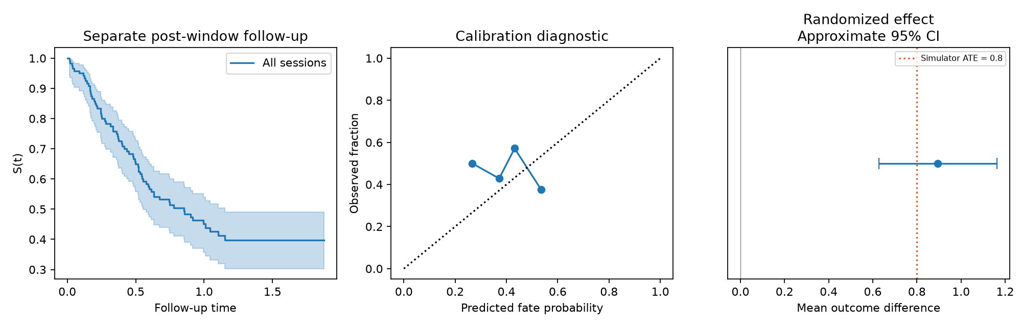
Kaplan–Meier summarizes the cohort descriptively. A penalized Cox model uses baseline risk and treatment, trains on training sessions, and evaluates on held-out sessions. Its concordance is about 0.515, providing weak ranking evidence in this tiny test. Concordance is not survival-probability calibration. Neither this toy fit nor the plotted curve is a validated clinical or product forecast.
Prediction is not an intervention
User interest can affect both narrative state and dropout. Then a state-dropout association partly reflects a common cause. For a prompt treatment $A$, define potential outcomes $Y(1)$ and $Y(0)$ and an average treatment effect
$$ \operatorname{ATE}=E[Y(1)-Y(0)]. $$Only one potential outcome is observed per unit. Random assignment makes the groups comparable in expectation. Under consistency and no interference, the group mean difference estimates the randomized treatment effect. The lab generates a separate continuous outcome
$$ Y=0.7\,\text{baseline}+0.8A+\text{noise}. $$Its true ATE is 0.8. The seeded estimate is 0.895, with an approximate independent-group 95% interval [0.627, 1.163]. This estimate concerns that continuous outcome, not the fate classifier or the Cox hazard coefficient. The interval expresses sampling uncertainty under this synthetic design; it does not validate a real prompt intervention.
For an A/B test, define assignment unit, treatment, outcome, and horizon before examining results. Repeated sessions from one user may require user-level assignment and dependence-aware uncertainty. The simulator’s sessions are independent units. Hernán and Robins, Causal Inference: What If
Observational alternatives need their own assumptions
A propensity score is $e(L)=P(A=1\mid L)$ for pretreatment covariates $L$. Weighting or matching can balance measured covariates, but a causal interpretation also requires conditional exchangeability, positivity, and consistency. It cannot balance an unmeasured confounder by definition. Adjusting for a post-treatment state can change the causal question or introduce bias.
Difference-in-differences compares changes:
$$ \widehat\tau=(\bar Y_{\mathrm{treated,post}}-\bar Y_{\mathrm{treated,pre}}) -(\bar Y_{\mathrm{control,post}}-\bar Y_{\mathrm{control,pre}}). $$Its central assumption concerns untreated counterfactual trends: without treatment, the groups would have changed in parallel. Absence of a significant pretrend does not prove this condition. Anticipation, changing composition, or concurrent interventions can undermine the design. The lab implements a randomized comparison, not propensity adjustment or DiD. Kahn-Lang and Lang on DiD assumptions
Exercises and the final project
- Censoring: recompute the four-record example after mistakenly labeling the record at 3 as an event. Answer: the curve incorrectly falls to $1/2$ at 3, then $1/4$ at 4. Explain what information was invented.
- Prediction: move the prefix cutoff from 0.4 to 0.7 and refit all preprocessing. Hint: a later landmark may expose branch information, but this changes the prediction task. Report both landmarks without claiming that the later result solves early forecasting.
- Causality: suppose a new prompt is given only to already disengaged users. Is a worse observed outcome proof of harm? Answer: no. Baseline disengagement confounds assignment; randomization or justified identification assumptions are needed.
For the final character-conversation project, define a prediction landmark and endpoint before feature extraction. Deliver a state representation, a geometry or graph diagnostic, one trajectory or dynamics baseline, and a session-level held-out outcome analysis. Include a shuffled-order or constant-prediction control, uncertainty, and one failure case. Distinguish observed associations from any separately designed intervention estimate. If no suitable real dataset is available, complete the same report on the provided synthetic data and label its scope explicitly.
The full chain is now useful because each arrow has a testable role: representation → geometry → graph → trajectory → dynamics → fate. A successful project explains which links the data support and where additional observations or an experiment are still needed.